Complexity
Introduction to Complexity
In the previous unit, we considered which computational problems are solvable by algorithms, without any constraints on the time and memory used by the algorithm. We saw that even with unlimited resources, many problems—indeed, “most” problems—are not solvable by any algorithm.
In this unit on computational complexity, we consider problems that are solvable by algorithms, and focus on how efficiently they can be solved. Primarily, we will be concerned how much time it takes to solve a problem. [1] We mainly focus on decision problems—i.e., languages—then later broaden our treatment to functional—i.e., search—problems.
A Turing machine’s running time, also known as time complexity, is the number of steps it takes until it halts; similarly, its space complexity is the number of tape cells it uses. We focus primarily on time complexity, and as previously discussed, we are interested in the asymptotic complexity with respect to the input size, in the worst case. For any particular asymptotic bound \(\O(t(n))\), we define the set of languages that are decidable by Turing machines having time complexity \(\O(t(n))\), where \(n\) is the input size:
Define
The set \(\DTIME(t(n))\) is an example of a complexity class: a set of languages whose complexity in some metric of interest is bounded in some specified way. Concrete examples include \(\DTIME(n)\), the class of languages that are decidable by Turing machines that run in (at most) linear \(O(n)\) time; and \(\DTIME(n^2)\), the class of languages decidable by quadratic-time Turing machines.
When we discussed computability, we defined two classes of languages: the decidable languages (also called recursive), denoted by \(\RD\), and the recognizable languages (also called recursively enumerable), denoted by \(\RE\). The definitions of these two classes are actually model-independent: they contain the same languages, regardless of whether our computational model is Turing machines, lambda calculus, or some other sensible model, as long as it is Turing-equivalent.
Unfortunately, this kind of model independence does not extend to \(\DTIME(t(n))\). Consider the concrete language
In a computational model with random-access memory, or even in the two-tape Turing-machine model, \(\PALINDROME\) can be decided in linear \(\O(n)\) time, where \(n = \abs{x}\): just walk pointers inward from both ends of the input, comparing character by character.
However, in the standard one-tape Turing-machine model, it can be proved that there is no \(\O(n)\)-time algorithm for \(\PALINDROME\); in fact, it requires \(\Omega(n^2)\) time to decide. Essentially, the issue is that an algorithm to decide this language would need to compare the first and last symbols of \(x\), which requires moving the head sequentially over the entire string, and do similarly for second and second-to-last symbols of \(x\), and so on. Because \(n/4\) of the pairs require moving the head by at least \(n/2\) cells each, this results in a total running time of \(\Omega(n^2)\). [2] So, \(\PALINDROME \notin \DTIME(n)\), but in other computational models, \(\PALINDROME\) can be decided in \(\O(n)\) time.
A model-dependent complexity class is very inconvenient, because we wish to analyze algorithms at a higher level of abstraction, without worrying about the details of the underlying computational model, or how the algorithm would be implemented on it, like the particulars of data structures (which can affect asymptotic running times).
Polynomial Time and the Class \(\P\)
We wish to define a complexity class that captures all problems that can be solved “efficiently”, and is also model-independent. As a step toward this goal, we note that there is an enormous qualitative difference between the growth of polynomial functions versus exponential functions. The following illustrates how several polynomials in \(n\) compare to the exponential function \(2^n\):

The vertical axis in this plot is logarithmic, so that the growth of \(2^n\) appears as a straight line. Observe that even a polynomial with a fairly large exponent, like \(n^{10}\), grows much slower than \(2^n\) (except for small \(n\)), with the latter exceeding the former for all \(n \geq 60\).
In addition to the dramatic difference in growth between polynomials and exponentials, we also observe that polynomials have nice closure properties: if \(f(n),g(n)\) are polynomially bounded, i.e., \(f(n) = \O(n^c)\) and \(g(n) = \O(n^{c'})\) for some constants \(c,c'\), then
are polynomially bounded as well, because \(\max\set{c,c'}\), \(c+c'\), and \(c \cdot c'\) are constants. These facts can be used to prove that if we compose a polynomial-time algorithm that uses some subroutine with a polynomial-time implementation of that subroutine, then the resulting full algorithm is also polynomial time. This composition property allows us to obtain polynomial-time algorithms in a modular way, by designing and analyzing individual components in isolation.
Thanks to the above properties of polynomials, it has been shown that the notion of polynomial-time computation is “robust” across many popular computational models, like the many variants of Turing machines, lambda calculi, etc. That is, any of these models can simulate any other one with only polynomial “slowdown”. So, any particular problem is solvable in polynomial time either in all such models, or in none of them.
The above considerations lead us to define “efficient” to mean “polynomial time (in the input size)”. From this we get the following model-independent complexity class of languages that are decidable in polynomial time (across many models of computation).
The complexity class \(\P\) is defined as
In other words, a language \(L \in \P\) if it is decided by some Turing machine that runs in time \(O(n^k)\) for some constant \(k\).
In brief, \(\P\) is the class of “efficiently decidable” languages. Based on what we saw in the algorithms unit, this class includes many fundamental problems of interest, like the decision versions of the greatest common divisor problem, sorting, the longest increasing subsequence problem, etc. Note that since \(\P\) is a class of languages, or decision problems, it technically does not include the search versions of these problems—but see below for the close relationship between search and decision.
As a final remark, the extended Church-Turing thesis posits that the notion of polynomial-time computation is “robust” across all realistic models of computation:
A problem is solvable in polynomial time on a Turing machine if and only if it is solvable in polynomial time in any “realistic” model of computation.
Because “realistic” is not precisely defined, this is just a thesis, not a statement than can be proved. Indeed, this is a major strengthening of the standard Church-Turing thesis, and there is no strong agreement about whether it is even true! In particular, the model of quantum computation may pose a serious challenge to this thesis: it is known that polynomial-time quantum algorithms exist for certain problems, like factoring integers into their prime divisors, that we do not know how to solve in polynomial time on Turing machines! So, if quantum computation is “realistic”, and if there really is no polynomial-time factoring algorithm in the TM model, then the extended Church-Turing thesis is false. While both of these hypotheses seem plausible, they are still uncertain at this time: real devices that can implement the full model of quantum computation have not yet been built, and we do not have any proof that factoring integers (or any other problem that quantum computers can solve in polynomial time) requires more than polynomial time on a Turing machine.
Examples of Efficient Verification
For some computational problems, it is possible to efficiently verify whether a claimed solution is actually correct—regardless of whether computing a correct solution “from scratch” can be done efficiently. Examples of this phenomenon are abundant in everyday life, and include:
Logic and word puzzles like mazes, Sudoku, or crosswords: these come in various degrees of difficulty to solve, some quite challenging. But given a proposed solution, it is straightforward to check whether it satisfies the “rules” of the puzzle. (See below for a detailed example with mazes.)
Homework problems that ask for correct software code (with justification) or mathematical proofs: producing a good solution might require a lot of effort and creativity to discover the right insights. But given a candidate solution, one can check relatively easily whether it is clear and correct, simply by applying the rules of logic. For example, to verify a claimed mathematical proof, we just need to check whether each step follows logically from the hypotheses and the previous steps, and that the proof reaches the desired conclusion.
Music, writing, video, and other media: creating a high-quality song, book, movie, etc. might require a lot of creativity, effort, and expertise. But given such a piece of media, it is relatively easy for even a non-expert to decide whether it is engaging and worthwhile to them (even though this is a subjective judgment that may vary from person to person). For example, even though the authors of this text could not come close to writing a beautiful symphony or a hit pop song, we easily know one when we hear one.
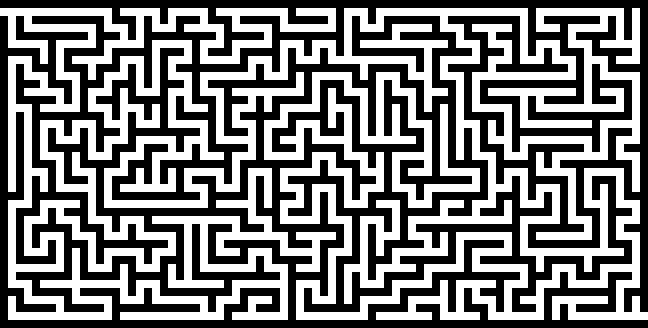
As a detailed example, consider the following maze, courtesy of Kees Meijer’s maze generator:
At first glance, it is not clear whether this maze has a solution. However, suppose that someone—perhaps a very good solver of mazes, or the person who constructed the maze—were to claim that this maze is indeed solvable. Is there some way that they could convince us of this fact?
A natural idea is simply to provide us with a path through the maze as “proof” of the claim. It is easy for us to check that this proof is valid, by verifying that the path goes from start to finish without crossing any “wall” of the maze. By definition, any solvable maze has such a path, so it is possible to convince us that a solvable maze really is solvable.
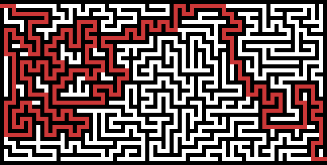
On the other hand, suppose that a given maze does not have a solution. Then no matter what claimed “proof” someone might give us, the checks we perform will cause us to reject it: because the maze is not solvable, any path must either fail to go from start to finish, or cross a wall somewhere (or both).
In summary: for any given maze, checking that a claimed solution goes from start to finish without crossing any wall is an efficient verification procedure:
The checks can be performed efficiently, i.e., in polynomial time in the size of the maze.
If the maze is solvable, then there exists a “proof”—namely, a path through the maze from start to finish—that the procedure will accept. How to find such a proof is not the verifier’s concern; all that matters is that it exists. [3]
If the maze is not solvable, then no claimed “proof” will satisfy the procedure.
Observe that we need both of the last two conditions in order for the procedure to be considered a correct verifier:
An “overly skeptical” verifier that cannot be “convinced” by anything, even though the maze is actually solvable, would not be correct.
Similarly, an “overly credulous” verifier that can be “fooled” into accepting, even when the maze is not solvable, would also be incorrect.
As already argued, our verification procedure has the right balance of “skepticism” and “credulity”.
As another example, the traveling salesperson problem (TSP) is the task of finding a minimum-weight tour of a given weighted graph. In this text, a “tour” of a graph is a cycle that visits every vertex exactly once, i.e., it is a path that visits every vertex and then immediately returns to its starting vertex. (Beware that some texts define “tour” slightly differently.) Without loss of generality, for TSP we can assume that the graph is complete—i.e., there is an edge between every pair of vertices—by filling in any missing edges with edges of enormous (or infinite) weight. This does not affect the solution(s), because any tour that uses any of these new edges will have larger weight than any tour that does not use any of them.
Suppose we are interested in a minimum-weight tour of the following graph:

If someone were to claim that the path \(A \to B \to D \to C \to A\) is a minimum-weight tour, could we efficiently verify that this is true? There doesn’t seem to be an obvious way to do so, apart from considering all other tours and checking whether any of them have smaller weight. While this particular graph only has three distinct tours (ignoring reversals and different starting points on the same cycle), in general, the number of tours in a graph is exponential in the number of vertices, so this approach would not be efficient. So, it is not clear whether we can efficiently verify that a claimed minimum-weight tour really is one.
However, let’s modify the problem to be a decision problem, which simply asks whether there is a tour whose total weight is within some specified “budget”:
Given a weighted graph \(G\) and a budget \(k\), does \(G\) have a tour of weight at most \(k\)?
Can the existence of such a tour be proved to an efficient, suitably skeptical verifier? Yes: simply provide such a tour as the proof. The verifier, given a path in \(G\)—i.e., a list of vertices—that is claimed to be such a tour, would check that all of the following hold:
the path starts and ends at the same vertex,
the path visits every vertex in the graph exactly once (except for the repeated start vertex at the end), and
the sum of the weights of the edges on the path is at most \(k\).
(All of these tests can be performed efficiently; see the formalization in Algorithm 144 below for details.)
For example, consider the following claimed “proofs” that the above graph has a tour that is within budget \(k=60\):
The path \(A \to B \to D \to C\) does not start and end at the same vertex, so the verifier’s first check would reject it as invalid.
The path \(A \to B \to D \to A\) starts and ends at the same vertex, but it does not visit vertex \(C\), so the verifier’s second check would reject it.
The path \(A \to B \to D \to C \to A\) satisfies the first two checks, but it has total weight \(61\), which is not within the budget, so the verifier’s third check would reject it.
The path \(A \to B \to C \to D \to A\) satisfies the first two checks, and its total weight of \(58\) is within the budget, so the verifier would accept it.
These examples illustrate that when the graph has a tour that is within the budget, there are still “proofs” that are “unconvincing” to the verifier—but there will also be a “convincing” proof, which is what matters to us.
On the other hand, it turns out that the above graph does not have a tour that is within a budget of \(k=57\). And for this graph and budget, the verifier will reject no matter what claimed “proof” it is given. This is because every tour in the graph—i.e., every path that would pass the verifier’s first two checks—has total weight at least \(58\).
In general, for any given graph and budget, the above-described verification procedure is correct:
If there is a tour of the graph that is within the budget, then there exists a “proof”—namely, such a tour itself—that the procedure will accept. (As before, how to find such a proof is not the verifier’s concern.)
If there is no such tour, then no claimed “proof” will satisfy the procedure, i.e., it cannot be “fooled” into accepting.
Efficient Verifiers and the Class \(\NP\)
We now generalize the above examples to formally define the notion of “efficient verification” for an arbitrary decision problem, i.e., a language. This definition captures the notion of an efficient procedure that can be “convinced”—by a suitable “proof”—to accept any string in the language, but cannot be “fooled” into accepting a string that is not in the language.
An efficient verifier for a language \(L\) is a Turing machine \(V(x,c)\) that takes two inputs, an instance \(x\) and a certificate (or “claimed proof”) \(c\) whose size \(\abs{c}\) is polynomial in \(\abs{x}\), and satisfies the following properties:
Efficiency: \(V(x,c)\) runs in time polynomial in its input size. [4]
Completeness: if \(x \in L\), then there exists some \(c\) for which \(V(x,c)\) accepts.
Soundness: if \(x \notin L\), then for all \(c\), \(V(x,c)\) rejects.
Alternatively, completeness and soundness together are equivalent to the following property (which is often more natural to prove for specific verifiers):
Correctness: \(x \in L\) if and only if there exists some \(c\) (of size polynomial in \(\abs{x}\)) for which \(V(x,c)\) accepts.
We say that a language is efficiently verifiable if there is an efficient verifier for it.
The claimed equivalence can be seen by taking the contrapositive of the soundness condition, which is: if there exists some \(c\) for which \(V(x,c)\) accepts, then \(x \in L\). (Recall that when negating a predicate, “for all” becomes “there exists”, and vice-versa.) This contrapositive statement and completeness are, respectively, the “if” and “only if” parts of correctness.
We sometimes say that a certificate \(c\) is “valid” or “invalid” for a given instance \(x\) if \(V(x,c)\) accepts or rejects, respectively. Note that the decision of the verifier is what determines whether a certificate is “(in)valid”—not the other way around—and that the validity of a certificate depends on both the instance and the verifier. There can be many different verifiers for the same language, which in general can make different decisions on the same \(x,c\) (though they all must reject when \(x \notin L\)).
In general, the instance \(x\) and certificate \(c\) are arbitrary strings over the verifier’s input alphabet \(\Sigma\) (and they are separated on the tape by some special character that is not in \(\Sigma\), but is in the tape alphabet \(\Gamma\)). However, for specific languages, \(x\) and \(c\) will typically represent various mathematical objects like integers, arrays, graphs, vertices, etc. As in the computability unit, this is done via appropriate encodings of the objects, denoted by \(\inner{\cdot}\), where without loss of generality every string decodes as some object of the desired “type” (e.g., integer, list of vertices, etc.). Therefore, when we write the pseudocode for a verifier, we can treat the instance and certificate as already having the desired types.
Discussion of Completeness and Soundness
We point out some of the important aspects of completeness and soundness (or together, correctness) in Definition 139.
Notice some similarities and differences between the notions of verifier and decider (Definition 61):
When the input \(x \in L\), both kinds of machine must accept, but a verifier need only accept for some value of the certificate \(c\), and may reject for others. By contrast, a decider does not get any other input besides \(x\), and simply must accept it.
When the input \(x \notin L\), both kinds of machine must reject, and moreover, a verifier must reject for all values of \(c\).
There is an asymmetry between the definitions of completeness and soundness:
If a (sound) verifier for language \(L\) accepts some input \((x,c)\), then we can correctly conclude that \(x \in L\), by the contrapositive of soundness. (A sound verifier cannot be “fooled” into accepting an instance that is not in the language.)
However, if a (complete) verifier for \(L\) rejects some input \((x,c)\), then in general we cannot reach any conclusion about whether \(x \in L\): it might be that \(x \notin L\), or it might be that \(x \in L\) but \(c\) is just not a valid certificate for \(x\). (In the latter case, by completeness, some other certificate \(c'\) is valid for \(x\).)
In summary, while every string \(x \in L\) has a “convincing proof” of its membership in \(L\), a string \(x \notin L\) does not necessarily have a proof of its non-membership in \(L\).
Discussion of Efficiency
We also highlight some important but subtle aspects of the notion of efficiency from Definition 139.
First, we restrict certificates \(c\) to have size that is some polynomial in the size of the instance \(x\), i.e., \(\abs{c}=O(\abs{x}^k)\) for some constant \(k\). The specific polynomial can depend on the verifier, but the same polynomial bounds the certificate size for all instances of the language. We make this restriction because we want verification to be efficient in every respect. It would not make sense to allow certificates to be (say) exponentially long in the instance size, since even reading such a long certificate should not be considered “efficient.”
We emphasize that merely requiring the verifier to have polynomial running time (in the size of the input) would not prohibit such pathological behavior. This is because the verifier’s input is both the instance \(x\) and certificate \(c\). For example, consider a certificate that consists of all the exponentially many tours in a graph. The verifier could check all of them in time linear in the certificate size, and hence linear in the size of its input. But this is not efficient in the sense we want, because it takes exponential time in the size of the graph.
With the above in mind, an equivalent definition of verifier efficiency, without any explicit restriction on the certificate size, is “running time polynomial in the size of the instance \(x\) alone”—not the entire input \(x,c\). Such a verifier can read only polynomially many of the initial symbols of \(c\), because reading each symbol and moving the head takes a computational step. So, the rest of the certificate (if any) is irrelevant, and can be truncated without affecting the verifier’s behavior. Therefore, we can assume without loss of generality that the certificate size is polynomial in the size of the instance \(x\), as we do in Definition 139 above.
The Class \(\NP\)
With the notion of an efficient verifier in hand, analogously to how we defined \(\P\) as the class of efficiently decidable languages, we define \(\NP\) as the class of efficiently verifiable languages.
The complexity class \(\NP\) is defined as the set of efficiently verifiable languages:
In other words, a language \(L \in \NP\) if there is an efficient verifier for it, according to Definition 139. [5]
Let us now formalize our first example of efficient verification from above: the decision problem of determining whether a given maze has a solution. A maze can be represented as an undirected graph, with a vertex for each “intersection” in the maze (along with the start and end points), and edges between adjacent positions. So, the decision problem is to determine whether, given such a graph, there exists a path from the start vertex \(s\) to the end vertex \(t\). This can be represented as the language [6]
We define an efficient verifier for \(\MAZE\) as follows; the precise pseudocode is given in Algorithm 141. An instance is a graph \(G = (V,E)\), a start vertex \(s\), and a target vertex \(t\). A certificate is a sequence of up to \(\abs{V}\) vertices in the graph. (This limit on the number of vertices in the certificate can be enforced by the decoding, and it ensures that the certificate size is polynomial in the instance size; see the Discussion of Efficiency.) The verifier checks that the sequence describes a valid path in the graph from \(s\) to \(t\), i.e., that the first and last vertices in the sequence are \(s\) and \(t\) (respectively), and that there is an edge between every pair of consecutive vertices in the sequence.
VerifyMAZE is an efficient verifier for \(\MAZE\), so \(\MAZE \in \NP\).
We show that VerifyMAZE satisfies Definition 139 by showing that it is efficient and correct.
First, VerifyMAZE runs in time polynomial in the size \(\abs{G} \geq \abs{V}\) of the graph: it compares two vertices from the certificate against the start and end vertices in the instance, and checks whether there is an edge between up to \(\abs{V}-1\) pairs of consecutive vertices in the certificate. Each pair of vertices can be checked in polynomial time. The exact polynomial depends on the representation of \(G\) and the underlying computational model, but it is polynomial in any reasonable representation (e.g., adjacency lists, adjacency matrix), which is all that matters for our purposes here.
As for correctness:
If \((G,s,t) \in \MAZE\), then by definition there is some path \(s = v_1 \to v_2 \to \dots \to v_{m-1} \to v_m = t\) in \(G\) that visits \(m \leq \abs{V}\) vertices in total, because any cycle in the path can be removed. Then by inspection of the pseudocode, VerifyMAZE\(((G, s, t), c = (v_1, v_2, \ldots, v_{m}))\) accepts.
Conversely, if VerifyMAZE\(((G,s,t), c = (v_1, \ldots, v_m))\) accepts for some certificate \(c\), then by inspection of the pseudocode, \(c\) represents a path from \(v_1=s\) to \(v_m=t\) in \(G\), so \((G,s,t) \in \MAZE\) by definition.
Alternatively, instead of showing the “conversely” part of correctness as above, we could have argued that VerifyMAZE is sound, as follows: if \((G,s,t) \notin \MAZE\), then by definition there is no path between \(s\) and \(t\) in \(G\), so any certificate \(c\) will either not start at \(s\), not end at \(t\), or it will have some pair of consecutive vertices with no edge between them. Thus, by inspection of the pseudocode, VerifyMAZE\(((G, s, t), c)\) will reject.
This kind of reasoning is correct, but it is more cumbersome and error prone, since it involves more cases and argues about the non-existence of certain objects. Usually, and especially for more complex verifiers, it is easier and more natural to directly prove the correctness condition (\(x \in L\) if and only if there exists \(c\) such that \(V(x,c)\) accepts) instead of soundness.
Next, returning to the “limited-budget” TSP example, we define the corresponding language
A certificate for a given instance \((G=(V,E),k)\) is a sequence of up to \(\abs{V}\) vertices in the graph. The verifier simply checks that the vertices form a tour whose cost is at most \(k\). The precise pseudocode is given in Algorithm 144.
VerifyTSP is an efficient verifier for \(\TSP\), so \(\TSP \in \NP\).
We show that VerifyTSP satisfies Definition 139 by showing that it is efficient and correct.
First, VerifyTSP runs in time polynomial in the size \(\abs{G,k}\) of the instance: checking for duplicate vertices \(v_i, v_j\) can be done in polynomial time, e.g., by checking all \(O(m^2) = O(\abs{V}^2)\) pairs of distinct \(1 \leq i,j \leq m\). Then the algorithm loops over \(\abs{V}\) edges, summing their weights. These weights are included in the input instance, so they can be summed in polynomial time in the instance size. Finally, the algorithm compares the sum against \(k\), which can be done in polynomial time.
We now argue correctness:
If \((G, k) \in \TSP\), then by definition, \(G\) has a tour of weight at most \(k\). Let \(c\) be the sequence of \(\abs{V}+1\) vertices in such a tour, starting and ending at the same arbitrary vertex, which has size polynomial in \(\abs{G}\). By inspection, we see that VerifyTSP\(((G,k),c)\) accepts, because all of \(V\)’s checks are satisfied by this \(c\).
Conversely, if VerifyTSP\(((G,k),c)\) accepts for some \(c = (v_0, \ldots, v_m)\), then because all of \(V\)’s checks are satisfied, this \(c\) starts and ends at the same vertex \(v_0=v_{m}\), it visits all \(\abs{V}\) vertices exactly once (because there are no duplicate vertices among \(v_1, \ldots, v_m\)), and the total weight of all \(m\) edges between consecutive vertices in \(c\) is at most \(k\). Therefore, \(c\) is a tour of \(G\) having total weight at most \(k\), hence \((G,k) \in \TSP\), as needed.
P Versus NP
We have defined two complexity classes:
\(\P\) is the class of languages that can be decided efficiently.
\(\NP\) is the class of languages that can be verified efficiently.
More precisely, a language \(L \in \P\) if there exists a polynomial-time algorithm \(D\) such that:
if \(x \in L\), then \(D(x)\) accepts;
if \(x \notin L\), then \(D(x)\) rejects.
Similarly, \(L \in \NP\) if there exists a polynomial-time algorithm \(V\) such that:
if \(x \in L\), then \(V(x, c)\) accepts for at least one (poly-sized) certificate \(c\);
if \(x \notin L\), then \(V(x, c)\) rejects for all certificates \(c\).
How are these two classes related? First, if a language is efficiently decidable, then it is also efficiently verifiable, trivially: the verifier can just ignore the certificate, and determine on its own whether the input is in the language, using the given efficient decider. (As an exercise, formalize this argument according to the definitions.) This gives us the following result.
\(\P \subseteq \NP\).
The above relationship allows for two possibilities:
\(\P \subsetneq \NP\), i.e., \(\P\) is a proper subset of (hence not equal to) \(\NP\); or
\(\P = \NP\).
The latter possibility would mean that every efficiently verifiable problem is also efficiently decidable. Is this the case? What is the answer to the question
We do not know the answer to this question! Indeed, the “\(\P\) versus \(\NP\)” question is perhaps the greatest open problem in Computer Science—and even one of the most important problems in all of Mathematics, as judged by the Clay Mathematics Institute, which has offered a $1 million prize for its resolution.
Consider the two example languages from above, \(\MAZE\) and \(\TSP\). We saw that both are in \(\NP\), and indeed, they have similar definitions, and their verifiers also have much in common. However, we know that \(\MAZE \in \P\): it can be decided efficiently simply by checking whether a breadth-first search from vertex \(s\) reaches vertex \(t\). On the other hand, we do not know whether \(\TSP\) is in \(\P\): we do not know of any efficient algorithm that decides \(\TSP\), and we do not know how to prove that no such algorithm exists. Most experts believe that there is no efficient algorithm for \(\TSP\), which would imply that \(\P \neq \NP\), but the community has no idea how to prove this.
How could we hope to resolve the \(\P\)-versus-\(\NP\) question? To show that the two classes are not equal, as most experts believe, it would suffice to demonstrate that some single language is in \(\NP\), but is not in \(\P\). However, this seems exceedingly difficult to do: we would need to somehow prove that, of all the infinitely many efficient algorithms—including many we have not yet discovered and cannot even imagine—none of them decides the language in question. [7] On the other hand, showing that \(\P = \NP\) also seems very difficult: we would need to demonstrate that every one of the infinitely many languages in \(\NP\) can be decided efficiently, i.e., by some polynomial-time algorithm.
Fortunately, a rich theory has been developed that will make the resolution of \(\P\) versus \(\NP\) (somewhat) simpler. As we will see below, it is possible to prove that some languages in \(\NP\) are the “hardest” ones in that class, in the following sense:
an efficient algorithm for any one of these “hardest” languages would imply an efficient algorithm for every language in \(\NP\)!
So, to prove that \(\P = \NP\), it would suffice to prove that just one of these “hardest” languages is in \(\P\). And in the other direction, the most promising route to prove \(\P \neq \NP\) is to show that one of these “hardest” languages is not in \(\P\)—because if some \(\NP\) language is not in \(\P\), then the same goes for all these “hardest” languages in \(\NP\).
In summary, the resolution of the \(\P\)-versus-\(\NP\) question lies entirely with the common fate of these “hardest” languages:
Any one of them has an efficient algorithm, if and only if all of them do, if and only if \(\P=\NP\).
Conversely, any one of them does not have an efficient algorithm, if and only if none of them do, if and only if \(\P \neq \NP\).
It turns out that there are thousands of known “hardest” languages in \(\NP\). In fact, as we will see, \(\TSP\) is one of them! We will prove this via a series of results, starting with the historically first language that was shown to be one of the “hardest” in \(\NP\), next.
Satisfiability and the Cook-Levin Theorem
Our first example of a “hardest” problem in \(\NP\) is the satisfiability problem for Boolean formulas. Given as input a Boolean formula like
we wish to determine whether there is a true/false assignment to its variables that makes the formula evaluate to true. Let us define the relevant terms:
a (Boolean) variable like \(x\) or \(y\) or \(x_{42}\) can be assigned the value “true” (often represented as 1) or “false” (represented as 0);
a literal is either a variable or its negation, e.g., \(x\) or \(\neg y\);
an operator is either conjunction (AND), represented as \(\wedge\); disjunction (OR), represented as \(\vee\); or negation (NOT), represented either as \(\neg\) or with an overline, like \(\neg(x \wedge y)\) or, equivalently, \(\overline{x \wedge y}\).
A Boolean formula is a well-formed mathematical expression involving literals combined with operators, and following the usual rules of parentheses for grouping.
An initial observation is that using the rules of logic like De Morgan’s laws, we can eliminate any double-negations, and we can iteratively move all negations “inward” to the literals, e.g., \(\neg (x \wedge \neg y) = (\neg x \vee y)\). So, from now on we assume without loss of generality that the negation operator appears only in literals.
We define the size of a formula to be the number of literals it has, counting duplicate appearances of the same literal. [8] For example, the formula \(\phi\) above has size 6. Note that the size of a formula is at least the number of distinct variables that appear in the formula.
An assignment is a mapping of the variables in a formula to truth values. We can represent an assignment over \(n\) variables (under some fixed order) as an \(n\)-tuple, such as \((a_1, \ldots, a_n)\). For the above formula, the assignment \((0, 1, 0)\) maps \(x\) to the value 0 (false), \(y\) to the value 1 (true), and \(z\) to the value 0 (false). The notation \(\phi(a_1, \dots, a_n)\) denotes the value of \(\phi\) when evaluated on the assignment \((a_1, \dots, a_n)\), i.e., with each variable substituted by its assigned value.
(More generally, we can also consider a partial assignment, which maps a subset of the variables to truth values. Evaluating a formula on a partial assignment is denoted like \(\phi(x=0, y=1)\), which assigns \(x\) to false and \(y\) to true; this yields another formula in the remaining variables.)
A satisfying assignment for a formula is an assignment that makes the formula evaluate to true. In the above example, \((0, 1, 0)\) is a satisfying assignment:
On the other hand, \((1, 0, 1)\) is not a satisfying assignment:
A formula \(\phi\) is satisfiable if it has at least one satisfying assignment. The decision problem of determining whether a given formula is satisfiable corresponds to the following language.
The (Boolean) satisfiability language is defined as
A first observation is that \(\SAT\) is decidable. A formula \(\phi\) of size \(n\) has at most \(n\) variables, so there are at most \(2^n\) possible assignments. Therefore, we can decide \(\SAT\) using a brute-force algorithm that simply iterates over all of the assignments of its input formula, accepting if at least one of them satisfies the formula, and rejecting otherwise. Although this is not efficient, it is apparent that it does decide \(\SAT\).
We also observe that \(\SAT\) has an efficient verifier, so it is in \(\NP\).
\(\SAT \in \NP\).
A certificate, or “claimed proof”, for a formula \(\phi\) is just an assignment for its variables. The following efficient verifier simply evaluates the given formula on the given assignment and accepts if the value is true, otherwise it rejects.
For efficiency, first observe that the size of the certificate is polynomial (indeed, linear) in the size of the instance \(\phi\), because it consists of a true/false value for each variable that appears in the formula. This verifier runs in linear time in the size of its input formula \(\phi\), because evaluating each AND/OR operator in the formula reduces the number of terms in the expression by one.
For correctness, by the definitions of \(\SAT\) and \(V_{\SAT}\),
so by Definition 139, \(V_{\SAT}\) is indeed an efficient verifier for \(\SAT\), as claimed.
Is \(\SAT\) efficiently decidable?—i.e., is \(\SAT \in \P\)? The decider we described above is not efficient: it takes time exponential in the number of variables in the formula, and the number of variables may be as large as the size of the formula (i.e., the number of literals in it), so in the worst case the algorithm runs in exponential time in its input size.
However, the above does not prove that \(\SAT \notin \P\); it just shows that one specific (and naïve) algorithm for deciding \(\SAT\) is inefficient. Conceivably, there could be a more sophisticated efficient algorithm that cleverly analyzes an arbitrary input formula in some way to determine whether it is satisfiable. Indeed, there are regular conferences and competitions to which researchers submit their best ideas, algorithms, and software for solving \(\SAT\). Although many algorithms have been developed that perform very impressively on large \(\SAT\) instances of interest, none of them is believed to run in polynomial time and to be correct on all instances.
To date, we actually do not know whether \(\SAT\) is efficiently decidable—we do not know an efficient algorithm for it, and we do not know how to prove that no such algorithm exists. Yet although the question of whether \(\SAT \in \P\) is unresolved, the Cook-Levin Theorem says that \(\SAT\) is a “hardest” problem in \(\NP\). [9]
If \(\SAT \in \P\), then every \(\NP\) language is in \(\P\), i.e., \(\P=\NP\).
The full proof of the Cook-Levin Theorem is ingenious and rather intricate, but its high-level idea is fairly easy to describe. Let \(L\) be an arbitrary language in \(\NP\); this means there is an efficient verifier \(V\) for \(L\). Using the hypothesis that \(\SAT \in \P\), we will construct an efficient decider for \(L\), which implies that \(L \in \P\), as claimed.
The key idea behind the efficient decider for \(L\) is that, using just the fact that \(V\) is an efficient verifier for \(L\), we can efficiently transform any instance of \(L\) into an instance of \(\SAT\) that has the same “yes/no answer”: either both instances are in their respective languages, or neither is. More precisely, there is an efficient procedure that maps any instance \(x\) of \(L\) to a corresponding Boolean formula \(\phi_{V,x}\), such that [10]
By the hypothesis that \(\SAT \in \P\), there is an efficient decider \(D_{\SAT}\) for \(\SAT\), so from all this we get the following efficient decider for \(L\):
Since \(\phi_{V,x}\) can be constructed in time polynomial in the size of \(x\), and \(D_\SAT\) runs in time polynomial in the size of \(\phi_{V,x}\), by composition, \(D_L\) as a whole runs in time polynomial in the size of \(x\). And the fact that \(D_L\) is correct (i.e., it decides \(L\)) follows directly from the correctness of \(D_{\SAT}\) and the above-stated relationship between \(x\) and \(\phi_{V,x}\).
This completes the high-level description of the proof strategy. In the following section we show how to efficiently construct \(\phi_{V,x}\) from \(x\), so that they satisfy the above-stated relationship.
Proof of the Cook-Levin Theorem
Configurations and Tableaus
In order to describe the construction of \(\phi_{V,x}\), we fist need to recall the notion of a configuration of a Turing machine and its representation as a sequence, which we previously discussed in Wang Tiling. A configuration encodes a “snapshot” of a Turing machine’s execution: the contents of the machine’s tape, the active state \(q \in Q\), and the position of the tape head. We represent these as an infinite sequence over the alphabet \(\Gamma \cup Q\) (the union of the finite tape alphabet and the TM’s finite set of states), which is simply:
the contents of the tape, in order from the leftmost cell,
with the active state \(q \in Q\) inserted directly to the left of the symbol corresponding to the cell on which the head is positioned.
For example, if the input is \(x_1 x_2 \cdots x_n\) and the initial state is \(q_0\), then the following sequence represents the machine’s starting configuration:
Since the head is at the leftmost cell and the state is \(q_0\), the string has \(q_0\) inserted to the left of the leftmost tape symbol. If the transition function gives \(\delta(q_0, x_1) = (q', x', R)\), then the next configuration is represented by
The first cell’s symbol has been changed to \(x'\), the machine is in state \(q'\), and the head is at the second cell, represented here by writing \(q'\) to the left of that cell’s symbol.
As stated above in the proof overview, for any language \(L \in \NP\) there exists an efficient verifier \(V\) that takes as input an instance \(x\), a certificate \(c\) whose size is some polynomial in \(\abs{x}\), and which runs in time polynomial in the input size, and hence in \(\abs{x}\) as well. So altogether, there is some constant \(k\) such that \(V(x, c)\) runs for at most \(\abs{x}^k\) steps before halting, for any \(x,c\). [11] Since the head starts at the leftmost cell and can move only one position in each step, this implies that \(V(x, c)\) can read or write only the first \(\abs{x}^k\) cells of the tape. Thus, instead of using an infinite sequence, we can represent any configuration during the execution of \(V(x,c)\) using just a finite string of length about \(\abs{x}^k\), ignoring the rest since it cannot affect the execution.
For an instance \(x\) of size \(n=\abs{x}\), we can represent the sequence of all the configurations of the machine, over its (at most) \(n^k\) computational steps, as an \(n^k\)-by-\(n^k\) tableau, with one configuration per row; for convenience later on, we also place a special \(\#\) symbol at the start and end of each row. [12] So, each cell of the tableau contains a symbol from the set \(S = \Gamma \cup Q \cup \set{\#}\), where \(\Gamma\) is the finite tape alphabet of \(V\); \(Q\) is the finite set of states in \(V\); and \(\# \notin \Gamma \cup Q\) is a special extra symbol.

Observe that, since \(V\) is deterministic, the contents of the first row of the tableau completely determine the contents of all the rows, via the “code” of \(V\). Moreover, adjacent rows represent a single computational step of the machine, and hence are identical to each other, except in the vicinity of the symbols representing the active states before and after the transition. Finally, \(V(x,c)\) accepts if and only if the accept-state symbol \(\qacc \in Q\) appears somewhere in its tableau. These are important feature of tableaus that are exploited in the construction of the formula \(\phi_{V,x}\), which we describe next.
Constructing the Formula
With the notion of a computational tableau in hand, we now describe the structure of the formula \(\phi_{V,x}\) that is constructed from the instance \(x\) (also using the fixed code of \(V\)).
The variables of the formula represent the contents of all the cells in a potential tableau for \(V\). That is, assigning Boolean values to all the variables fully specifies the contents of a claimed tableau, including the value of a certificate \(c\) in the first row.
Conceptually, we can think of an assignment to the variables, and the potential tableau that they represent, as a claimed execution transcript for \(V\).
The formula \(\phi_{V,x}\) is carefully designed to evaluate whether the claimed tableau (as specified by the variables’ values) meets two conditions:
it is the actual execution tableau of \(V(x,c)\), for the specific given instance \(x\), and whatever certificate \(c\) appears in the first row, and
it is an accepting tableau, i.e., \(V(x,c)\) accepts.
Conceptually, we can think of \(\phi_{V,x}\) as checking whether the claimed execution transcript for \(V\) is genuine, and results in \(V\) accepting the specific instance \(x\).
In summary, the formula \(\phi_{V,x}\) evaluates to true if and only if its variables are set so that they specify the full and accepting execution tableau of \(V(x,c)\), for the certificate \(c\) specified by the variables. Therefore, as needed,
where the last equivalence holds by Definition 139.
We now give the details. The variables of the formula are as follows:
For each cell position \(i,j\) of the tableau, and each symbol \(s \in S\), there is a Boolean variable \(t_{i,j,s}\).
So, there are \(\abs{S} \cdot n^{2k} = O(n^{2k})\) variables in total, which is polynomial in \(n = \abs{x}\) because \(\abs{S}\) and \(2k\) are constants. (Recall that \(S\) is a fixed finite alphabet that does not vary with \(n\).)
Assigning Boolean values to these variables specifies the contents of a claimed tableau, as follows:
Assigning \(t_{i,j,s} = \text{true}\) specifies that cell \(i,j\) of the claimed tableau has symbol \(s\) in it.
Observe that the variables can be assigned arbitrary Boolean values, so for the same cell location \(i,j\), we could potentially assign \(t_{i,j,s} = \text{true}\) for multiple different values of \(s\), or none at all. This would make the contents of cell \(i,j\) undefined. The formula \(\phi_{V,x}\) is designed to “check” for this and evaluate to false in such a case, and also to check for all the other needed properties on the claimed tableau, as we now describe.
The formula \(\phi_{V,x}\) is defined as the conjunction (AND) of four subformulas:
Each subformula “checks” (or “enforces”) a certain condition on the variables and the claimed tableau they specify, evaluating to true if the condition holds, and false if it does not. The subformulas check the following conditions:
\(\phi_{\text{cell}}\) checks that each cell of the claimed tableau is well defined, i.e., it contains exactly one symbol;
\(\phi_{\text{accept}}\) checks that the claimed tableau is an accepting tableau, i.e., that \(\qacc\) appears somewhere in it;
\(\phi_{\text{start},x}\) checks that the first row of the claimed tableau is valid, i.e., it represents the initial configuration of the verifier running on the given instance \(x\) and some certificate \(c\) (as specified by the variables);
\(\phi_{\text{move},V}\) checks that each non-starting row of the claimed tableau follows from the previous one, according to the transition function of \(V\).
Observe that, as needed above, all these conditions hold if and only if the claimed tableau is indeed the actual accepting execution tableau of \(V(x,c)\), for the certificate \(c\) that appears in the first row. So, it just remains to show how to design the subformulas to correctly check their respective conditions, which we do next.
Cell Consistency
To check that a given cell \(i,j\) has a well-defined symbol, we need exactly one of the variables \(t_{i,j,s}\) to be true, over all \(s \in S\). The formula
checks that at least one of the variables is true, and the formula
checks that no more than one of the variables is true (where the equality holds by De Morgan’s laws).
Putting these together over all cells \(i,j\), the subformula
checks that for all \(i,j\), exactly one of \(t_{i,j,s}\) is true, as needed.
The formula has \(\O(\abs{S}^2) = O(1)\) literals for each cell (because \(S\) is a fixed alphabet that does not vary with \(n=\abs{x}\)), so \(\phi_{\text{cell}}\) has size \(\O(n^{2k})\), which is polynomial in \(n=\abs{x}\) because \(2k\) is a constant.
Accepting Tableau
To check that the claimed tableau is an accepting one, we just need to check that at least one cell has \(\qacc\) as its symbol, which is done by the following subformula:
This has one literal per cell, for a total size of \(\O(n^{2k})\), which again is polynomial in \(n=\abs{x}\).
Starting Configuration
For the top row of the tableau, which represents the starting configuration, we suppose that the encoding of an input pair \((x, c)\) separates \(x\) from \(c\) on the tape using a special symbol \(\$ \in \Gamma \setminus \Sigma\) that is in the tape alphabet \(\Gamma\) but not in the input alphabet \(\Sigma\). (Recall that \(x\) and \(c\) are strings over \(\Sigma\), so \(\$\) unambiguously separates them.) Letting \(m=\abs{c}\), the top row of the tableau is therefore as follows:

The row starts with the \(\#\) symbol. Since the machine is in active state \(\qst\), and the head is at the leftmost cell of the tape, \(\qst\) is the second symbol. The contents of the tape follow, which are the symbols of the input \(x\), then the \(\$\) separator, then the symbols of the certificate \(c\), then blanks until we have \(n^k\) symbols, except for the last symbol, which is \(\#\).
We now describe the subformula \(\phi_{\text{start},x}\) that checks that the first row of the claimed tableau has the above form. We require the row to have the specific, given instance \(x\) in its proper position of the starting configuration. This is checked by the formula
For the tableau cells corresponding to the certificate, our construction does not know what certificate(s) \(c\), if any, would cause \(V(x,c)\) to accept, or even what their sizes are (other than that they are less than \(n^k\)). Indeed, a main idea of this construction is that any satisfying assignment for \(\phi_{V,x}\), if one exists, specifies a valid certificate \(c\) for \(x\) (and vice versa).
So, our formula allows any symbol \(s \in \Sigma \cup \set{\bot}\) from the input alphabet, as well as blank, to appear in the positions after the separator \(\$\). We just need to ensure that any blanks appear only after the certificate string, i.e., not before any symbol from \(\Sigma\). Overall, the formula that checks that the portion of the first row dedicated to the certificate is well-formed is
In words, this says that each cell in the zone dedicated to the certificate either has a blank, or has an input-alphabet symbol and the preceding symbol is not blank.
Putting these pieces together with the few other fixed cell values, the subformula that checks the first row of the claimed tableau is:
This subformula has one literal for each symbol in the instance \(x\), the start state, and the special \(\#\) and \(\$\) symbols. It has \(O(\abs{\Sigma}) = O(1)\) literals for each cell in the zone dedicated to the certificate (recall that the tape alphabet \(\Gamma\) is fixed and does not vary with \(n=\abs{x}\)). Thus, this subformula has size \(\O(n^k)\), which again is polynomial in \(n=\abs{x}\).
Transitions
Finally, we describe the subformula that checks whether every non-starting row in the claimed tableau follows from the previous one. This is the most intricate part of the proof, and the only one that relies on the transition function, or “code”, of \(V\).
As a warmup first attempt, recall that any syntactically legal configuration string \(r\) (regardless of whether \(V\) can actually reach that configuration) determines the next configuration string \(r'\), according to the code of \(V\). So, letting \(i,i+1\) denote a pair of adjacent row indices, and \(r\) denote a legal configuration string, we could write:
the formula that checks whether row \(i\) equals \(r\) and row \(i+1\) equals the corresponding \(r'\), namely,
\[\large \phi_{i,r} = \bigwedge_{j=1}^{n^k} (t_{i,j,r_j} \wedge t_{i+1,j,r'_j}) \; \text;\]the formula that checks whether row \(i+1\) follows from row \(i\), namely,
\[\large \phi_i = \bigvee_{\text{legal } r} \phi_{i,r} \; \text;\]the formula that checks whether every non-starting row follows from the previous one, namely,
\[\large \phi_{\text{move},V} = \bigwedge_{i=1}^{n^k-1} \phi_i \; \text.\]
Because \(\phi_{\text{start},x}\) checks that the first row of the claimed tableau is a valid starting configuration, \(\phi_{\text{start},x} \wedge \phi_{\text{move},V}\) does indeed check that the entire claimed tableau is valid.
This approach gives a correct formula, but unfortunately, it is not efficient—the formula does not have size polynomial in \(n=\abs{x}\). The only problem is in the second step: because there are multiple valid choices for each symbol of a legal \(r\), and \(r\) has length \(n^k\), there are exponentially many such \(r\). So, taking the OR over all of them results in a formula of exponential size.
To overcome this efficiency problem, we proceed similarly as above, but using a finer-grained breakdown of adjacent rows than in \(\phi_{i,r}\) above. The main idea is to consider the 2-by-3 “windows” (subrectangles) of adjacent rows, and check that every window is “valid” according to the code of \(V\). It can be proved that if all the overlapping 2-by-3 windows of a claimed pair of rows are valid, then the pair as a whole is valid. This is essentially because valid adjacent rows are almost identical (except around the cells with the active states), and the windows overlap sufficiently to guarantee that any invalidity in the claimed rows will be exposed in some 2-by-3 window. [13]

There are \(\abs{S}^6 = O(1)\) distinct possibilities for a 2-by-3 window, but not all of them are valid. Below we describe all the valid windows, and based on this we construct the subformula \(\phi_{\text{move},V}\) as follows.
For any particular valid window \(w\), let \(s_1, \ldots, s_6\) be its six symbols, going left-to-right across its first then second row. Similarly to \(\phi_{i,r}\) above, the following simple formula checks whether the window of the claimed tableau with top-left corner at \(i,j\) matches \(w\):
Now, letting \(W\) be the set of all valid windows, similarly to \(\phi_i\) above, the following formula checks whether the window at \(i,j\) of the claimed tableau is valid:
Finally, we get the subformula that checks whether every window in the tableau is valid:
The set \(W\) of valid windows has size \(\abs{W} \leq \abs{S}^6 = O(1)\), so each \(\phi_{i,j}\) has \(O(1)\) literals. Because there are \(\O(n^{2k})\) windows to check, the subformula \(\phi_{\text{move},V}\) has size \(\O(n^{2k})\), which again is polynomial in \(n=\abs{x}\).
We now describe all the valid windows. The precise details of this are not so essential, because all we used above were the facts that the valid windows are well defined, and that there are \(O(1)\) of them. We use the following notation in the descriptions and diagrams:
\(\gamma\) for an arbitrary element of \(\Gamma\),
\(q\) for an arbitrary element of \(Q\),
\(\rho\) for an arbitrary element of \(\Gamma \cup Q\),
\(\sigma\) for an arbitrary element of \(\Gamma \cup \set{\#}\).
First, a window having the \(\#\) symbol somewhere in it is valid only if \(\#\) is in the first position of both rows, or is in the third position of both rows. So, every valid window has one of the following forms, where the symbols \(\rho_1, \dots, \rho_6\) must additionally be valid according to the rules below.

If a window is not in the vicinity of a state symbol \(q \in Q\), then the machine’s transition does not affect the portion of the configuration corresponding to the window, so the top and bottom rows match:

To reason about what happens in a window that is in the vicinity of a state symbol, we consider how the configuration changes as a result of a right-moving transition \(\delta(q, \gamma) = (q', \gamma', R)\):

The head moves to the right, so \(q'\) appears in the bottom row at the column to the right of where \(q\) appears in the top row. The symbol \(\gamma\) is replaced by \(\gamma'\), though its position moves to the left to compensate for the rightward movement of the state symbol. There are four windows affected by the transition, labeled above by their leftmost columns. We thus have the following four kinds of valid windows corresponding to a rightward transition \(\delta(q, \gamma) = (q', \gamma', R)\):

Note that we have used \(\sigma\) for the edges of some windows, as there can be either a tape symbol or the tableau-edge marker \(\#\) in these positions.
We now consider how the configuration changes as a result of a left-moving transition \(\delta(q, \gamma) = (q', \gamma', L)\):

The head moves to the left, so \(q'\) appears in the bottom row at the column to the left of where \(q\) appears in the top row. As with a rightward transition, we replace the old symbol \(\gamma\) with the new symbol \(\gamma'\). This time, however, the symbol to the left of the original position of the head moves right to compensate for the leftward movement of the head. So here we have the following five kinds of valid windows corresponding to the leftward transition \(\delta(q, \gamma) = (q', \gamma', R)\):

We also need to account for the case where the head is at the leftmost cell on the tape, in which case the head does not move:

Here we have three kinds of valid windows, but the last one actually has the same structure as the last window in the normal case for a leftward transition. Thus, we have only two more kinds of valid windows:

Finally, we need one last set of valid windows to account for the machine reaching the accept state before the last row of the tableau. As stated above, the valid tableau is “padded” with copies of the final configuration, so the valid windows for this case look like:

Conclusion
We summarize the main claims about what we have just done.
Using an efficient verifier \(V\) for an arbitrary language \(L \in \NP\), we have demonstrated how to efficiently construct a corresponding formula \(\phi_{V,x}\) from a given instance \(x\) of \(L\). The formula can be constructed in time polynomial in \(\abs{x}\), and in particular the total size of the formula is \(\O(\abs{x}^{2k})\) literals.
Then, we (almost entirely) proved that \(x \in L \iff \phi_{V,x} \in \SAT\). In the \(\implies\) direction: by correctness of \(V\), any \(x \in L\) has at least one certificate \(c\) that makes \(V(x,c)\) accept, so the computation tableau for \(V(x,c)\) is accepting. In turn, by design of the formula \(\phi_{V,x}\), this tableau defines a satisfying assignment for the formula (i.e., an assignment to its variables that makes \(\phi_{V,x}\) evaluate to true). So, \(x \in L\) implies that \(\phi_{V,x} \in \SAT\).
In the \(\impliedby\) direction: if the constructed formula \(\phi_{V,x} \in \SAT\), then by definition it has a satisfying assignment. Again by the special design of the formula, any satisfying assignment defines the contents of an actual accepting computation tableau for \(V(x,c)\), for the \(c\) appearing in the top row of the tableau. Since \(V(x,c)\) accepts for this \(c\), we conclude that \(x \in L\) by the correctness of the verifier. So, \(\phi_{V,x} \in \SAT\) implies that \(x \in L\).
Finally, if \(\SAT \in \P\), then an efficient decider \(D_\SAT\) for \(\SAT\) exists, and we can use it to decide \(L\) efficiently: given an instance \(x\), simply construct \(\phi_{V,x}\) and output \(D_\SAT(\phi_{V,x})\); by the above property, this correctly determines whether \(x \in L\). As a result, \(\SAT \in \P\) implies that \(\NP \subseteq \P\) and hence \(\P = \NP\), as claimed.
\(\NP\)-Completeness
With the example of \(\SAT\) and the Cook-Levin theorem in hand, we now formally define what it means to be a “hardest” problem in \(\NP\), and demonstrate several examples of such problems.
Polynomial-Time Mapping Reductions
The heart of the Cook-Levin theorem is an efficient algorithm for converting an instance of an (arbitrary) language \(L \in \NP\) to an instance \(\phi_{V,x}\) of \(\SAT\), such that
Thus, any (hypothetical) efficient decider for \(\SAT\) yields an efficient decider for \(L\), which simply converts its input \(x\) to \(\phi_{V,x}\) and invokes the decider for \(\SAT\) on it.
This kind of efficient transformation, from an arbitrary instance of one problem to a corresponding instance of another problem having the same “yes/no answer”, is known as a polynomial-time mapping reduction, which we now formally define.
A polynomial-time mapping reduction—also known as a Karp reduction for short—from a language \(A\) to a language \(B\) is a function \(f \colon \Sigma^* \to \Sigma^*\) having the following properties: [14]
Efficiency: \(f\) is polynomial-time computable: there is an algorithm that, given any input \(x \in \Sigma^*\), outputs \(f(x)\) in time polynomial in \(\abs{x}\).
Correctness: for all \(x \in \Sigma^*\),
\[x \in A \iff f(x) \in B \; \text.\]Equivalently, if \(x \in A\) then \(f(x) \in B\), and if \(x \notin A\) then \(f(x) \notin B\). [15]
If such a reduction exists, we say that \(A\) polynomial-time mapping-reduces (or Karp-reduces) to \(B\), and write \(A \leq_p B\).

We first observe that a polynomial-time mapping reduction is essentially a special case of (or more precisely, implies the existence of) a Turing reduction: we can decide \(A\) by converting the input instance of \(A\) to an instance of \(B\) using the efficient transformation function, then querying an oracle that decides \(B\). The following makes this precise.
If \(A \leq_p B\), then \(A \leq_T B\).
Because \(A \leq_p B\), there is an efficiently computable function \(f\) such that \(x \in A \iff f(x) \in B\). To show that \(A \leq_T B\), we give a Turing machine \(M_A\) that decides \(A\) using an oracle \(M_B\) that decides \(B\):
Clearly, \(M_A\) halts on any input, because \(f\) is polynomial-time computable and \(M_B\) halts on any input. And by the correctness of \(M_B\) and the code of \(M_A\),
Therefore, \(M_A\) decides \(A\), by Definition 61.
Observe that the Turing reduction given in Proof 154 simply:
applies an efficient transformation to its input,
invokes its oracle once, on the resulting value, and
immediately outputs the oracle’s answer.
In fact, several (but not all!) of the Turing reductions we have seen for proving undecidability (e.g., for the halts-on-empty language and other undecidable languages) are essentially polynomial-time mapping reductions, because they have this exact form. (To be precise, the efficient transformation in such a Turing reduction is the mapping reduction, and its use of its oracle is just fixed “boilerplate”.)
Although a polynomial-time mapping reduction is essentially a Turing reduction, the reverse does not hold in general, due to some important differences:
A Turing reduction has no efficiency constraints, apart from the requirement that it halts: the reduction may run for arbitrary finite time, both before and after its oracle call(s).
By contrast, in a polynomial-time mapping reduction, the output of the conversion function must be computable in time polynomial in the input size.
A Turing reduction is a Turing machine that decides one language given an oracle (“black box”) that decides another language, which it may use arbitrarily. In particular, it may invoke the oracle multiple times (or not at all), and perform arbitrary “post-processing” on the results, e.g., negate the oracle’s answer.
By contrast, a polynomial-time mapping reduction does not involve any explicit oracle; it is merely a conversion function that must “preserve the yes/no answer”. Therefore, there is no way for it to “make multiple oracle calls,” nor for it to “post-process” (e.g., negate) the yes/no answer for its constructed instance. Implicitly, a polynomial-time mapping reduction corresponds to making just one oracle call and then immediately outputting the oracle’s answer. [16]
In Lemma 98 we saw that if \(A \leq_T B\) and \(B\) decidable, then \(A\) is also decidable. Denoting the class of decidable languages by \(\RD\), this result can be restated as:
If \(A \leq_T B\) and \(B \in \RD\), then \(A \in \RD\).
Polynomial-time mapping reductions give us an analogous result with respect to membership in the class \(\P\).
If \(A \leq_p B\) and \(B \in \P\), then \(A \in \P\).
Because \(B \in \P\), there is a polynomial-time Turing machine \(M_B\) that decides \(B\). And because \(A \leq_p B\), the Turing machine \(M_A\) defined in Proof 154, with the machine \(M_B\) as its “oracle”, decides \(A\).
In addition, \(M_A(x)\) runs in time polynomial in its input size \(\abs{x}\), by composition of polynomial-time algorithms. Specifically, by the hypothesis \(A \leq_p B\), computing \(f(x)\) runs in time polynomial in \(\abs{x}\), and as already noted, \(M_B\) runs in time polynomial in its input length, so the composed algorithm \(M_A\) runs in polynomial time.
Since \(M_A\) is a polynomial-time Turing machine that decides \(A\), we conclude that \(A \in \P\), as claimed.
Analogously to how Lemma 100 immediately follows from Lemma 98, the following corollary is merely the contrapositive of Lemma 155.
If \(A \leq_p B\) and \(A \notin \P\), then \(B \notin \P\).
\(\NP\)-Hardness and \(\NP\)-Completeness
With the notion of a polynomial-time mapping (or Karp) reduction in hand, the heart of the Cook-Levin theorem can restated as saying that
\(A \leq_p \SAT\) for every language \(A \in \NP\).
Combining this with Lemma 155, as an immediate corollary we get the statement of Theorem 151: if \(\SAT \in \P\), then every \(\NP\) language is in \(\P\), i.e., \(\P=\NP\).
Informally, the above says that \(\SAT\) is “at least as hard as” every language in \(\NP\) (under Karp reductions). This is a very important property that turns out to be shared by many languages, so we define a special name for it.
A language \(L\) is \(\NP\)-hard if \(A \leq_p L\) for every language \(A \in \NP\).
We define \(\NPH = \set{L : L \text{ is $\NP$-hard}}\) to be the class of all such languages.
We stress that a language need not be in \(\NP\), or even be decidable, to be \(\NP\)-hard. For example, it can be shown that the undecidable language \(\atm\) is \(\NP\)-hard (see Exercise 167).
With the notion of \(\NP\)-hardness in hand, the core of the Cook-Levin theorem is as follows.
\(\SAT\) is \(\NP\)-hard.
Previously, we mentioned the existence of languages that are, informally, the “hardest” ones in \(\NP\), and that \(\SAT\) was one of them. We now formally define this notion.
A language \(L\) is \(\NP\)-complete if:
\(L \in \NP\), and
\(L\) is \(\NP\)-hard.
We define \(\NPC = \set{L : L \text{ is $\NP$-complete}}\) to be the class of all such languages.
Since \(\SAT \in \NP\) (by Lemma 149) and \(\SAT\) is \(\NP\)-hard (by Cook-Levin), \(\SAT\) is indeed \(\NP\)-complete.
To show that some language \(L\) of interest is \(\NP\)-hard, do we need to repeat and adapt all the work of the Cook-Levin theorem, with \(L\) in place of \(\SAT\)? Thankfully, we do not! Analogously to Lemma 100—which lets us prove undecidability by giving a Turing reduction from a known-undecidable language—the following lemma shows that we can establish \(\NP\)-hardness by giving a Karp reduction from a known-\(\NP\)-hard language. (We do this below for several concrete problems of interest, in More NP-complete Problems.)
If \(A \leq_p B\) and \(A\) is \(\NP\)-hard, then \(B\) is \(\NP\)-hard.
This follows from the fact that \(\leq_p\) is a transitive relation; see Exercise 165 below. By the two hypotheses and Definition 158, \(L \leq_p A\) for every \(L \in \NP\), and \(A \leq_p B\), so \(L \leq_p B\) by transitivity. Since this holds for every \(L \in \NP\), by definition we have that \(B\) is \(\NP\)-hard, as claimed.
Combining Lemma 155, Lemma 157, and Lemma 161, the fact that \(A \leq_p B\) has the following implications in various scenarios.
Hypothesis |
Implies |
\(A \in \P\) |
nothing |
\(A \notin \P\) |
\(B \notin \P\) |
\(A\) is \(\NP\)-hard |
\(B\) is \(\NP\)-hard |
\(B \in \P\) |
\(A \in \P\) |
\(B \notin \P\) |
nothing |
\(B\) is \(\NP\)-hard |
nothing |
Resolving \(\P\) versus \(\NP\)
The concepts of \(\NP\)-hardness and \(\NP\)-completeness are powerful tools for making sense of, and potentially resolving, the \(\P\)-versus-\(\NP\) question. As the following theorem shows, the two possibilities \(\P = \NP\) and \(\P \neq \NP\) each come with a variety of equivalent “syntactically weaker” conditions. So, resolving \(\P\) versus \(\NP\) comes down to establishing any one of these conditions—which is still a very challenging task! In addition, the theorem establishes strict relationships between the various classes of problems we have defined, under each of the two possibilities \(\P = \NP\) and \(\P \neq \NP\).
The following statements are equivalent, i.e., if any one of them holds, then all of them hold.
Some \(\NP\)-hard language is in \(\P\).
(In set notation: \(\NPH \cap \P \neq \emptyset\).)
Every \(\NP\)-complete language is in \(\P\).
(In set notation: \(\NPC \subseteq \P\).)
\(\P = \NP\).
(In words: every language in \(\NP\) is also in \(\P\), and vice-versa.)
Every language, except the “trivial” languages \(\Sigma^*\) and \(\emptyset\), is \(\NP\)-hard. [17]
(In set notation: \(\mathcal{P}(\Sigma^*) \setminus \set{\Sigma^*, \emptyset} \subseteq \NPH\).)
It follows that \(\P \neq \NP\) if and only if no \(\NP\)-hard language is in \(\P\) (i.e., \(\NPH \cap \P = \emptyset\)), which holds if and only if some nontrivial language is not \(\NP\)-hard.
Before giving the proof of Theorem 163, we discuss its main consequences for attacking the \(\P\)-versus-\(\NP\) question. First, by the equivalence of Statements 1 and 2, all \(\NP\)-complete problems have the same “status” : either all of them are efficiently solvable—in which case \(\P=\NP\), by the equivalence with Statement 3—or none of them is, in which case \(\P \neq \NP\).
So, to prove that \(\P=\NP\), it would be sufficient (and necessary) to have an efficient algorithm for any single \(\NP\)-complete (or even just \(\NP\)-hard) problem. This is by the equivalence of Statements 1 and 3.
To prove that \(\P \neq \NP\), it would trivially suffice to prove that any single problem in \(\NP\) is not in \(\P\). For this we might as well focus our efforts on showing this for some \(\NP\)-complete problem, because by the equivalence of Statements 3 and 1, some \(\NP\) problem lacks an efficient algorithm if and only if every \(\NP\)-complete problem does.
Alternatively, to prove that \(\P \neq \NP\), by the equivalence of Statements 3 and 4 it would suffice to show that some nontrivial language in \(\NP\) is not \(\NP\)-hard. For this we might as well focus our efforts on showing this for some language in \(\P\), because by the equivalence of Statements 4 and 1, if any nontrivial language in \(\NP\) is not \(\NP\)-hard, then every nontrivial language in \(\P\) is not \(\NP\)-hard.
Based on Theorem 163, the following Venn diagram shows the necessary and sufficient relationships between the classes \(\P\), \(\NP\), \(\NP\)-hard (\(\NPH\)), and \(\NP\)-complete (\(\NPC\)), for each of the two possibilities \(\P \neq \NP\) and \(\P = \NP\).

We refer to Statement 1 as “S1”, and similarly for the others. The following implications hold immediately by the definitions (and set operations):
\(\text{S2} \implies \text{S1}\) because an \(\NP\)-complete, and hence \(\NP\)-hard, language exists (e.g., \(\SAT\)).
(In set notation: if \(\NPH \cap \NP = \NPC \subseteq \P\), then by intersecting with \(\P\), we get that \(\NPH \cap \P = \NPC \neq \emptyset\).)
\(\text{S3} \implies \text{S2}\) because by definition, every \(\NP\)-complete language is in \(\NP\).
(In set notation: if \(\P = \NP\), then \(\NPC \subseteq \NP \subseteq \P\).)
\(\text{S4} \implies \text{S1}\) because there is a nontrivial language \(L \in \P \subseteq \NP\) (e.g., \(L=\MAZE\)), and by S4, \(L\) is \(\NP\)-hard.
(In set notation: \(\emptyset \neq \P \setminus \set{\Sigma^*, \emptyset} \subseteq \NPH\), where the last inclusion is by S4, so by intersecting everything with \(\P\), we get that \(\emptyset \neq \P \setminus \set{\Sigma^*, \emptyset} \subseteq \NPH \cap \P\) and hence \(\NPH \cap \P \neq \emptyset\).)
So, to prove that each statement implies every other one, it suffices to show that \(\text{S1} \implies \text{S3} \implies \text{S4}\).
For \(\text{S1} \implies \text{S3}\), suppose that some \(\NP\)-hard language \(L\) is in \(P\). By definition, \(A \leq_p L\) for all \(A \in \NP\), so by Lemma 155, \(A \in \P\). Therefore, \(\NP \subseteq \P\), and this is an equality because \(\P \subseteq \NP\), as we have already seen.
For \(\text{S3} \implies \text{S4}\), suppose that \(\P = \NP\) and let \(L\) be an arbitrary nontrivial language; we show that \(L\) is \(\NP\)-hard. By nontriviality, there exist some fixed, distinct strings \(y \in L\) and \(z \notin L\). Let \(A \in \NP = \P\) be arbitrary, so there is an efficient algorithm \(M_A\) that decides \(A\). We show that \(A \leq_p L\) via the function \(f\) computed by the following pseudocode:
It is apparent that \(F\) is efficient, because \(M_A\) is. And for correctness, by the correctness of \(M_A\), the properties of \(y \neq z\), and the code of \(F\),
Since \(A \leq_p L\) for all \(A \in \NP\), we have shown that \(L\) is \(\NP\)-hard, as needed.
Show that polynomial-time mapping reductions are transitive. That is, if \(A \leq_p B\) and \(B \leq_p C\), then \(A \leq_p C\).
Show that no language Karp-reduces to \(\Sigma^*\) or to \(\emptyset\), except for \(\Sigma^*\) and \(\emptyset\) themselves (respectively). In particular, these languages are not \(\NP\)-hard, regardless of whether \(\P = \NP\).
Show that \(\atm\) is \(\NP\)-hard.
More \(\NP\)-Complete Problems
The Cook-Levin Theorem (Theorem 159, showing that \(\SAT\) is \(\NP\)-hard), together with the concept of polynomial-time mapping reductions and Lemma 161, are powerful tools for establishing the \(\NP\)-hardness of a wide variety of other natural problems. We do so for several such problems next.
3SAT
As a second example of an \(\NP\)-complete problem, we consider satisfiability of Boolean formulas having a special structure. First, we introduce some more relevant terminology.
A clause is a disjunction (OR) of literals, like \((a \vee \neg b \vee \neg c \vee d)\).
A Boolean formula is in conjunctive normal form (CNF) if it is a conjunction (AND) of clauses. An example of a CNF formula is
\[\phi = (a \vee b \vee \neg c \vee d) \wedge (\neg a) \wedge (a \vee \neg b) \wedge (c \vee d) \; \text.\]A 3CNF formula is a Boolean formula in conjunctive normal form where each clause has exactly three literals, like the following:
\[\phi = (a \vee b \vee \neg c) \wedge (\neg a \vee \neg a \vee d) \wedge (a \vee \neg b \vee d) \wedge (c \vee d \vee d) \; \text.\]Notice that clauses may have repeated literals, even though this has no effect on the satisfiability of the formula.
The 3CNF-satisfiability language is defined as the set of satisfiable 3CNF formulas:
Observe that every satisfiable 3CNF formula is a satisfiable Boolean formula, but not vice versa. Conceivably, the extra “structure” of 3CNF formulas might make it easier to decide whether they are satisfiable, as compared with general Boolean formulas. However, it turns out that this is not the case: the problem of deciding 3CNF satisfiability is \(\NP\)-complete. [18]
\(\TSAT\) is \(\NP\)-complete.
First, we must show that \(\TSAT \in \NP\). An efficient verifier for \(\TSAT\) is actually identical to the one for \(\SAT\), except that its input is a 3CNF formula. (As usual, the verifier interprets any input string as being an instance of the relevant language.)
By the same reasoning that applied to the verifier for \(\SAT\) (see Lemma 149), this is an efficient and correct verifier for \(\TSAT\).
We now show that \(\TSAT\) is \(\NP\)-hard, by proving that \(\SAT \leq_p \TSAT\). We do so by defining an efficient mapping reduction \(f\) that, given an arbitrary Boolean formula \(\phi\), outputs a 3CNF formula \(f(\phi)\) such that \(\phi \in \SAT \iff f(\phi) \in \TSAT\). The reduction \(f\) and its analysis are as follows.
First, convert \(\phi\) to a formula \(\phi'\) in conjunctive normal form that is satisfiable if and only if \(\phi\) is; we say that \(\phi\) and \(\phi'\) are equisatisfiable. (We stress that the formulas are not necessary equivalent, because they may have different variables.) We can perform this transformation efficiently, as described in detail below.
Then, convert the CNF formula \(\phi'\) to the output 3CNF formula \(f(\phi)\), as follows.
For each clause having more than three literals, split it into a pair of clauses by introducing a new “dummy” variable. Specifically, convert a clause
\[(l_1 \vee l_2 \vee \cdots \vee l_k)\]with \(k > 3\) literals into the two clauses
\[(z \vee l_1 \vee l_2) \wedge (\neg z \vee l_{3} \vee \cdots \vee l_k) \; \text,\]where \(z\) is some new variable that does not appear anywhere else in the formula. Observe that these two clauses have \(3\) and \(k-1\) literals, respectively, so the two new clauses both have strictly fewer literals than the original clause. [19] We thus repeat the splitting process until every clause has at most three literals.
We claim that each splitting preserves (un)satisfiability, i.e., the original formula before splitting and new CNF formula are equisatisfiable (i.e., either both are satisfiable, or neither is). Indeed, more generally, we claim that the formulas \((\rho \vee \rho')\) and \(\sigma = (z \vee \rho) \wedge (\neg z \vee \rho')\) are equisatisfiable for any formulas \(\rho,\rho'\) that do not involve variable \(z\).
In one direction, suppose that \(\sigma\) is satisfiable, i.e., it has a satisfying assignment \(\alpha\). Then the same assignment (ignoring the value of \(z\)) satisfies \((\rho \vee \rho')\), because \(\alpha\) makes exactly one of \(z,\neg z\) false, so it must make the corresponding one of \(\rho,\rho'\) true, and therefore satisfies \((\rho \vee \rho')\).
In the other direction, suppose that \((\rho \vee \rho')\) is satisfiable, i.e., it has a satisfying assignment \(\alpha\). Then \(\alpha\) leaves \(z\) unassigned (because \(z\) does not appear in \(\rho\) or \(\rho'\)), and it makes at most one of \(\rho,\rho'\) false; we therefore assign \(z\) to make the corresponding literal \(z\) or \(\neg z\) true. (If \(\alpha\) satisfies both \(\rho,\rho'\), we assign \(z\) arbitrarily.) This satisfies \(\sigma\) because it makes both of \((z \vee \rho)\) and \((\neg z \vee \rho')\) true.
Finally, for each clause that has fewer than three literals, expand it to have three literals simply by repeating its first literal. For example, the clause \((a)\) becomes \((a \vee a \vee a)\), and \((\neg b \vee c)\) becomes \((\neg b \vee \neg b \vee c)\). Trivially, this produces an equivalent formula in 3CNF form.
Each transformation on a clause can be done in constant time, and the total number of transformations is linear in the number of literals in (i.e., size of) \(\phi'\). This is because the splitting transformation transforms a clause having \(k > 3\) literals into a pair having \(3\) and \(k-1\) literals. So, the running time of this phase is linear in the size of \(\phi'\) (and in particular, the size of \(f(\phi)\) is linear in the size of \(\phi'\)).
Because both phases run in polynomial time in the length of their respective inputs, their composition runs in time polynomial in the length of the input formula \(\phi\), as needed. This completes the proof that \(\SAT \leq_p \TSAT\).
Clique
\(\NP\)-completeness arises in many problems beyond Boolean satisfiability. As an example, we consider the clique problem.
For an undirected graph \(G = (V, E)\), a clique is a subset \(C \subseteq V\) of the vertices for which there is an edge between every pair of (distinct) vertices in \(C\). Equivalently, the subgraph induced by \(C\), meaning the vertices in \(C\) and all the edges between them, is a complete graph.
The following is an example of a clique of size four, with the vertices of the clique and the edges between them highlighted:

We are often interested in finding a clique of maximum size in a graph, called a maximum clique for short. For instance, if a graph represents a group of people and their individual friend relationships, we might want to find a largest set of mutual friends—hence the name “clique”. However, this is not a decision problem; to obtain one, much like we did for the traveling salesperson problem, here we introduce a non-negative “threshold” parameter \(k\), which does not exceed the number of vertices in the graph (because no clique can exceed this size):
Since the search version of the clique problem is a maximization problem, the corresponding decision problem involves a lower bound on the clique size. Observe that if a graph has a clique of size at least \(k\), then it also has one of size exactly \(k\), because removing arbitrary vertices from a clique still results in a clique. In other words, any subset of a clique is itself a clique.
\(\CLIQUE\) is \(\NP\)-complete.
To prove the theorem, we show in the following two lemmas that \(\CLIQUE\) is in \(\NP\), and is \(\NP\)-hard.
\(\CLIQUE \in \NP\).
To prove the lemma we give an efficient verifier for \(\CLIQUE\), according to Definition 139. Our verifier takes an instance—i.e., a graph \(G\) and threshold \(k\)—and a certificate, which is a set of vertices that is claimed to be a clique of size \(k\) in the graph. The verifier simply checks whether this is indeed the case, i.e., whether the certificate has \(k\) vertices and there is an edge between each pair of these vertices.
We first analyze the running time of the verifier. The first check counts the number of vertices in the vertex subset \(C \subseteq V\), which runs in linear time in the size of the graph. Then the number of loop iterations is quadratic in the number of vertices, and each iteration can be done efficiently by looking up edges of the graph. So, the total running time is polynomial in the size of the instance, as needed.
We now prove the verifier’s correctness. We need to show that \((G,k) \in \CLIQUE\) if and only if there exists some (polynomial-size) \(C \subseteq V\) for which VerifyCLIQUE\(((G,k),C)\) accepts.
In one direction, if \((G, k) \in \CLIQUE\), then by definition there is some clique \(C \subseteq V\) of size \(k\), which is of size polynomial (indeed, linear) in the size of the instance \((G,k)\). In VerifyCLIQUE\(((G,k),C)\), all the checks pass because \(\abs{C}=k\) and there is an edge between every pair of vertices in \(C\). Thus, the verifier accepts \(((G, k), C)\), as needed.
Conversely, if VerifyCLIQUE\(((G,k),C)\) accepts for some certificate \(C \subseteq V\), then by the code of the verifier, \(\abs{C} = k\) and there is an edge between every pair of vertices in \(C\). So, by definition, \(C\) is a clique of size \(k\) in \(G\), hence \((G,k) \in \CLIQUE\), as needed.
\(\CLIQUE\) is \(\NP\)-hard.
To prove the lemma we will give a polynomial-time mapping reduction from the \(\NP\)-hard language \(\TSAT\). Before doing so, let’s review the definition of \(\TSAT\). An instance is a 3CNF formula, which is the AND of clauses that are each the OR of three literals:
Each literal \(\ell_i\) is either a variable itself (e.g., \(x\)) or its negation (e.g., \(\neg x\)). By definition, \(\TSAT\) is the language of all satisfiable 3CNF formulas; a formula is satisfiable if its variables can be assigned true/false values that make the formula evaluate to true.
Observe that a satisfying assignment simultaneously satisfies every clause, meaning that each clause has at least one literal that is true. So, a formula with \(m\) clauses is satisfiable if and only if there is some selection of \(m\) literals, one from each clause, that can simultaneously be made true under some assignment. This is a key fact we use in the reduction to \(\CLIQUE\).
We give a polynomial-time mapping reduction \(f\) from \(\TSAT\) to \(\CLIQUE\), showing that \(\TSAT \leq_p \CLIQUE\). Since \(\TSAT\) is \(\NP\)-hard, it follows that \(\CLIQUE\) is \(\NP\)-hard.
We need to define a polynomial-time computable function \(f\) that transforms a given 3CNF formula \(\phi\) into a corresponding instance \(f(\phi) = (G, k)\) of the clique problem, so that \(\phi \in \TSAT \iff f(\phi) \in \CLIQUE\). Given a 3CNF formula \(\phi\), the reduction constructs a \(\CLIQUE\) instance \((G,k)\) with graph \(G\) and threshold \(k\) defined as follows:
For each literal in \(\phi\), including duplicates, there is a corresponding vertex in \(G\). So, a formula with \(m\) clauses yields a graph \(G\) with exactly \(3m\) vertices.
For each pair of vertices in \(G\), there is an edge between them if their corresponding literals are in different clauses of \(\phi\), and are “consistent”—i.e., they can simultaneously be true. Specifically, two literals are consistent if they are not negations of each other (i.e., \(x\) and \(\neg x\) for some variable \(x\)). In other words, two literals are consistent if they are the same literal, or they involve different variables.
The threshold is set to \(k=m\), the number of clauses in \(\phi\).
For example, the following illustrates the graphs corresponding to two different formulas having three clauses each, where one formula is satisfiable and the other is unsatisfiable:

Observe that for the satisfiable formula on the left, the corresponding graph has a clique of size three (one such clique is highlighted), while the graph for the unsatisfiable formula on the right does not have a clique of size three.
We first show that the reduction is efficient. Creating one vertex per literal in the input formula takes linear time in the size of the formula, and creating the edges takes quadratic time, because for each pair of literals in different clauses, it takes constant time to determine whether they are consistent. So, the reduction is polynomial time in the size of the input formula.
We now prove that the reduction is correct. We need to show that \(\phi \in \TSAT \iff f(\phi) = (G,k) \in \CLIQUE\).
We first show that \(\phi \in \TSAT \implies (G,k) \in \CLIQUE\). Since \(\phi \in \TSAT\), it is satisfiable, which means there is some assignment \(\alpha\) under which each clause in \(\phi\) has at least one literal that is true. We show that there is a corresponding clique in \(G\) of size \(k=m\), the number of clauses in \(\phi\). Let \(s_1, s_2, \dots, s_m\) be a selection of one literal from each clause that is true under the assignment \(\alpha\). Then we claim that their corresponding vertices form a clique in \(G\):
Since all the literals \(s_i\) are true under assignment \(\alpha\), each pair of them is consistent, i.e., no two of them are a variable and its negation.
So, since all the literals \(s_i\) come from different clauses, each pair of their corresponding vertices has an edge between them, by construction of the graph.
Therefore, \(G\) has a clique of size \(k=m\), so \((G,k) \in \CLIQUE\), as needed.
We now show that converse, that \(f(\phi) = (G,k) \in \CLIQUE \implies \phi \in \TSAT\). It is important to understand that we are not “inverting” the function \(f\) here. Rather, we are showing that if the graph-threshold pair produced as the output of \(f(\phi)\) is in \(\CLIQUE\), then the input formula \(\phi\) must be in \(\TSAT\).
Since \(f(\phi) = (G, k=m) \in \CLIQUE\), the output graph \(G\) has some clique \(C = \set{c_1, \dots, c_m}\) of size \(m\). We show that \(\phi\) is satisfiable, by using the vertices in \(C\) to construct a corresponding assignment \(\alpha\) that satisfies \(\phi\).
Since \(C\) is a clique, there is an edge between every pair of vertices in \(C\). So, by the reduction’s construction of the graph, the vertices in \(C\) must correspond to consistent literals from different clauses.
Since there are \(m\) vertices in \(C\), they correspond to exactly one literal from each clause.
Since these literals are consistent, it is possible for all of them to be true simultaneously. That is, no two of these literals are a variable and its negation.
Therefore, we can define an assignment \(\alpha\) to the variables of \(\phi\) so that each literal corresponding to a vertex in \(C\) is true. That is, if a variable \(x\) is one such literal, we set \(x\) to be true; and if a negated variable \(\neg x\) is one such literal, we set \(x\) to be false. (Any variables that remain unset after this process can be set arbitrarily.) Since all the literals in question are consistent, the assignment is well defined; there is no conflict in setting them.
We can now see that \(\alpha\) is a satisfying assignment: the literals corresponding to the vertices in \(C\) are all true under \(\alpha\), and they collectively come from all \(m\) clauses, so \(\alpha\) satisfies \(\phi\). Thus \(\phi \in \TSAT\), as needed. This completes the proof.
It is worth remarking that the above reduction from \(\TSAT\) to \(\CLIQUE\) produces “special-looking” instances \((G,k)\) of \(\CLIQUE\): the graph \(G\) has exactly \(3k\) vertices, which are in groups of three where there is no edge among any such group. There is no issue with this: an (efficient) algorithm that solves \(\CLIQUE\) must be correct on special instances of this form (along with all others), so any such algorithm could also be used to (efficiently) solve \(\TSAT\) by applying the reduction to the input formula and invoking the \(\CLIQUE\) algorithm on the result. Indeed, the reduction implies that solving \(\CLIQUE\) even when it is restricted to such special instances is “at least as hard as” solving any problem in \(\NP\).
Vertex Cover
For an undirected graph \(G = (V, E)\), a vertex cover is a subset \(C \subseteq V\) of the vertices for which every edge in the graph is “covered” by a vertex in \(C\). An edge \(e = (u, v)\) is covered by \(C\) if at least one of its endpoints \(u,v\) is in \(C\). So, formally, \(C \subseteq V\) is a vertex cover for \(G\) if
The following are two vertex covers for the same graph:

The cover on the left has a size of five (vertices), while the cover on the right has a size of four.
Given a graph, we are interested in finding a vertex cover of minimum size, called a minimum vertex cover for short. Observe that \(V\) itself is a vertex cover in all case, though it may be far from optimal.
As a motivating example for the vertex-cover problem, consider a museum that consists of a collection of interconnected hallways, with exhibits on the walls. The museum needs to hire guards to monitor and protect the exhibits, but since guards are expensive, it seeks to minimize the number of guards while still ensuring that each hallway is protected by at least one guard. The museum layout can be represented as a graph, with the hallways as edges and the vertices as hallway intersections or endpoints. A guard placed at a vertex protects the exhibits in any of the hallways adjacent to that vertex. So, the museum wants to find a minimum vertex cover for this graph, to determine how many guards to hire and where to place them.
As we did for the traveling salesperson problem, we first define a decision version of the vertex cover problem, with a non-negative “budget” parameter \(k\) that does not exceed the number of vertices in the graph:
Since the search version of vertex cover is a minimization problem, the corresponding decision problem involves an upper bound (“budget”) on the vertex cover size. Observe that if a graph has a vertex cover of size less than \(k\), then it also has one of size exactly \(k\), simply by adding some arbitrary vertices. In other words, any superset of a vertex cover is also a vertex cover.
We now show that \(\VC\) is \(\NP\)-hard, leaving the proof that \(\VC \in \NP\) as an exercise. Combining these two results, we conclude that \(\VC\) is \(\NP\)-complete.
Show that \(\VC \in \NP\).
\(\VC\) is \(\NP\)-hard.
Before giving the formal proof, we first give the key ideas and an illustrative example. We will demonstrate a polynomial-time mapping reduction from the \(\NP\)-hard language \(\TSAT\): given a 3CNF formula, the reduction constructs a graph and a budget that corresponds to the formula in a certain way, so that the formula is satisfiable if and only if the graph has a vertex cover within the size budget.
The graph is made up of “gadget” subgraphs, one for each variable and clause in the formula. These are connected together with appropriate edges according to the contents of the formula.
A gadget for a variable \(x\) is a “barbell,” consisting of two vertices respectively labeled \(x\) and \(\neg x\), and connected by an edge. A gadget for a clause is a triangle whose three vertices are each labeled by a corresponding one of the literals. Example variable and clause gadgets are depicted here:

The reduction first creates one variable gadget for each variable, and one clause gadget for each clause. Then, it connects these gadgets using edges as follows: it adds an edge between each clause-gadget vertex and the (unique) variable-gadget vertex having the same literal label.
As a concrete example, consider the input formula
To construct the corresponding graph, we start with a gadget for each variable and clause:

Then, we connect each clause-gadget vertex to the variable-gadget vertex having the same literal label:

Observe that any vertex cover of the graph must cover each variable-gadget edge, so it must have at least one vertex from each variable gadget. Similarly, it must cover all three edges in each clause gadget, so it must have at least two vertices from each clause gadget. All this holds even ignoring the “crossing” edges that go between the variable and clause gadgets.
With this in mind, the reduction finally sets the budget to be \(k=n+2m\), where \(n\) is the number of variables and \(m\) is the number of clauses in the input formula. This corresponds to asking whether there is a vertex cover having no “additional” vertices beyond what is required by just the gadgets themselves. As the following proof shows, it turns out that there is a vertex cover of this size if and only if the input formula is satisfiable: any satisfying assignment of the formula yields a corresponding vertex cover of size \(k\), and vice versa.
For example, for the above example formula and corresponding graph, setting \(x = \text{true}\) and \(y = z = \text{false}\) satisfies the formula, and the graph has a corresponding vertex cover as depicted here:

Conversely, we can show that for any vertex cover of size \(k=n+2m\) in the graph, there is a corresponding satisfying assignment for \(\phi\), obtained by setting the variables so that the literals of all the variable-gadget vertices in the cover are true.
We give a polynomial-time mapping reduction from \(\TSAT\) to \(\VC\), showing that \(\TSAT \leq_p \VC\). Since \(\TSAT\) is \(\NP\)-hard, it follows that \(\VC\) is \(\NP\)-hard as well.
We need to define a polynomial-time computable function \(f\) that transforms a given 3CNF formula \(\phi\) into a corresponding instance \(f(\phi) = (G, k)\) of the vertex-cover problem, so that \(\phi \in \TSAT \iff (G,k) \in \VC\). The function \(f\) constructs \(G\) and \(k\) as follows:
For each variable \(x\) in \(\phi\), it creates a “variable gadget” consisting of two vertices, respectively labeled by the literals \(x\) and \(\neg x\), with an edge between them.
For each clause \((\ell_i \vee \ell_j \vee \ell_k)\) in \(\phi\), where \(\ell_i, \ell_j, \ell_k\) are literals, it creates a “clause gadget” consisting of three vertices, respectively labeled by these literals, with an edge between each pair of these vertices (i.e., a triangle).
For each vertex of each clause gadget, it creates an edge between that vertex and the (unique) variable-gadget vertex having the same label. That is, a clause-gadget vertex labeled by literal \(x\) (respectively, \(\neg x\)) has an edge to the variable-gadget vertex labeled \(x\) (respectively, \(\neg x\)).
Finally, set \(k=n+2m\) where \(n,m\) are respectively the number of variables and clauses in \(\phi\).
To see that the reduction is efficient, observe that there are \(2n + 3m\) vertices in \(G\), with \(n\) edges within the variable gadgets, \(3m\) edges within the clause gadgets, and \(3m\) edges that cross between the clause and variable gadgets, for a total of \(\O(m + n)\) edges. Thus, \(G\) has size \(\O(n + m)\), and it (along with \(k\)) can be constructed efficiently by iterating over the input formula \(\phi\).
We now show that the reduction is correct. We need to show that \(\phi \in \TSAT \iff f(\phi) = (G, n+2m) \in \VC\).
We first show that \(\phi \in \TSAT \implies f(\phi) = (G, n+2m) \in \VC\). In other words, if \(\phi\) is satisfiable, then \(G\) has a vertex cover of size \(n+2m\). Since \(\phi\) is satisfiable, there is some satisfying assignment \(\alpha\) under which each clause in \(\phi\) has at least one literal that is true. We show by construction that there is a corresponding vertex cover \(C\) of size \(n+2m\) in \(G\). We define \(C\) as follows:
For each variable gadget, include in \(C\) the vertex labeled by the literal that is true under \(\alpha\). That is, for each variable \(x\)’s gadget, place the vertex labeled by \(x\) in \(C\) if \(\alpha\) assigns \(x\) to be true, otherwise place the vertex labeled \(\neg x\) in \(C\).
Observe that exactly one vertex from each of the variable gadgets is in \(C\), and these \(n\) vertices cover all \(n\) of the variable-gadget edges.
In each clause gadget, observe that at least one of its three vertices is labeled by a literal that is true under \(\alpha\), because \(\alpha\) satisfies all the clauses in \(\phi\). Identifying an arbitrary one of these vertices per clause gadget, include in \(C\) the other two vertices of each gadget.
Observe that \(C\) has \(2m\) clause-gadget vertices, and these cover all \(3m\) of the clause-gadget edges.
As we have just seen, \(C\) has \(n+2m\) vertices in total, and covers all the edges that are “internal” to the gadgets. So, it just remains to show that \(C\) also covers all the “crossing” edges that go between the variable gadgets and clause gadgets.
To see this, recall that the crossing edges are those that go from each clause-gadget vertex \(v\) to the variable-gadget vertex having the same literal label \(\ell\). If \(v \in C\), then its crossing edge is covered by \(C\), so now suppose that \(v \notin C\). Then by construction of \(C\), \(v\)’s literal \(\ell\) is true under the assignment \(\alpha\). Therefore, the variable-gadget vertex labeled \(\ell\) is in \(C\), and hence \(v\)’s crossing edge is covered by \(C\). Because this reasoning holds for every clause-gadget vertex, all the crossing edges in \(G\) are covered by \(C\). We conclude that \(C\) is a vertex cover of \(G\), hence \((G,k) \in \VC\), as needed.
We now show the converse direction, that \((G, n+2m) \in \VC \implies \phi \in \TSAT\). In other words, if \(G\) has a vertex cover \(C\) of size at most \(n + 2m\), then \(\phi\) has a satisfying assignment. Indeed, we will show by construction that for any such \(C\), there is a corresponding satisfying assignment for \(\phi\).
As observed above, any vertex cover of \(G\) must have at least one vertex from each variable gadget (to cover that gadget’s edge), and at least two vertices from each clause gadget (to cover that gadget’s three edges). So, since \(C\) is a vertex cover of size at most \(n+2m\), it must have size exactly \(n+2m\), and therefore \(C\) has:
exactly one vertex from each variable gadget, and
exactly two vertices from each clause gadget.
Based on this, we define an assignment for \(\phi\) as follows: for each variable \(x\)’s gadget, identify which one of its vertices (labeled either \(x\) or \(\neg x\)) is in \(C\), and set the value of \(x\) so that the label of this vertex is true. That is, if the variable-gadget vertex labeled \(x\) is in \(C\), set \(x\) to be true; otherwise, set \(x\) to be false. (Note that this assignment is well defined because \(C\) has exactly one vertex from each variable gadget.)
We show that this assignment satisfies \(\phi\), using the fact that \(C\) is a vertex cover. Consider an arbitrary clause in \(\phi\); we claim that the assignment satisfies it (and hence the entire formula) because the clause has at least one true literal.
In the gadget corresponding to the clause, there is exactly one vertex \(v\) that is not in \(C\), which is labeled by some literal \(\ell\) that appears in the clause. Recall that the other endpoint of \(v\)’s “crossing edge” is the variable-gadget vertex having label \(\ell\). Since \(C\) covers this crossing edge, and \(v \notin C\), this other endpoint must be in \(C\). So by definition, \(\ell\) is set to true under the assignment. Finally, since \(\ell\) is one of the literals in the clause in question, the assignment satisfies the clause, as claimed. This completes the proof.
An independent set of an undirected graph \(G = (V, E)\) is a subset of the vertices \(I \subseteq V\) such that no two vertices in \(I\) have an edge between them. Define the language (with non-negative threshold \(k \leq \abs{V}\))
\[\IS = \set{(G, k) : G \text{ is an undirected graph with an independent set of size at least } k} \; \text.\]Show that \(\VC \leq_p \IS\).
Hint: If \(G\) has a vertex cover of size \(m\), what can be said about the vertices that are not in the cover?
Recall the language
\[\CLIQUE = \set{(G, k) : G \text{ is an undirected graph that has a clique of size at least $k$}} \; \text.\]Show that \(\IS \leq_p \CLIQUE\).
Set Cover
We now consider another problem, that of hiring workers for a project. To complete the project, we need workers that collectively have some set of skills. For instance, to build a house, we might need an architect, a general contractor, an engineer, an electrician, a plumber, a painter, and so on. There is a pool of candidate workers, where each worker has a certain set of skills. For example, there might be a worker who is proficient in plumbing and electrical work, another who can put up drywall and paint, etc. Our goal is to hire a team of workers of minimum size that “covers” all the required skills, i.e., for each skill, at least one hired worker has that skill.
We formalize this problem as follows. We are given an instance that consists of a set \(S\), representing the required skills, along with some subsets \(S_i \subseteq S\), representing the set of skills that each worker has. We wish to select as few of the \(S_i\) as possible to cover the set \(S\). In other words, we want to find a smallest set of indices \(C\) such that
As a concrete example, consider the following small instance:
There is no cover of size two: in order to cover skill \(5\), we must select subset \(S_5\) or \(S_6\), and no single subset covers all the remaining skills. However, there are several covers of size three. One example is \(C = \set{1, 2, 6}\), which gives us
We now define a language that corresponds to the decision version of the set-cover problem. As with vertex cover, we include a budget \(k\) for the size of the cover, which does not exceed the number of given subsets.
It is straightforward to show that \(\SC \in \NP\): a certificate is a set of indices \(C \subseteq \set{1,\ldots,n}\), and the verifier simply checks that \(\abs{C} \leq k\) and that \(\bigcup_{i\in C} S_i = S\), which can be done efficiently.
The following lemma shows that, like \(\TSAT\) and \(\VC\), \(\SC\) is a “hardest” problem in \(\NP\).
\(\SC\) is \(\NP\)-hard.
Before providing the formal proof, we give the key ideas and an illustrative example. First, we choose a suitable \(\NP\)-hard language to reduce from. While there are many choices that could work, it is preferable to choose a language that is “defined similarly” to the target language, because this typically makes the reduction and analysis simpler and less error prone.
For this reason, we will demonstrate a polynomial-time mapping reduction from the \(\NP\)-hard language \(\VC\). Given a \(\VC\) instance \((G = (V, E), k)\), the reduction needs to construct an \(\SC\) instance \((S, S_1, \ldots, S_n, k')\)—i.e., a set \(S\), subsets \(S_i \subseteq S\), and budget \(k'\)—so that \(G\) has a vertex cover of size (at most) \(k\) if and only if \(S\) can be covered by (at most) \(k'\) of the subsets.
To help conceive of such a reduction, it is first useful to identify the specific similarities between the \(\VC\) and \(\SC\) problems. The \(\VC\) problem asks to cover all the edges of a given graph by some limited number of its vertices budget, where each vertex covers its incident edges. The \(\SC\) problem asks to cover all the elements of a set (e.g., of skills) by a limited number of some given subsets (e.g., workers). So, a natural idea is for the reduction to generate a set that corresponds to the edges of the graph (these are the objects to be covered), and subsets that correspond to the vertices—specifically, each subset is the set of edges incident to its corresponding vertex. Because the vertices are in correspondence with the subsets, the reduction leaves the budget unchanged.
As an example, consider the following graph, where for convenience we have numbered the vertices and edges.

This graph has a vertex cover of size four, consisting of the vertices labeled with indices \(2,4,5,6\).
On this graph, the reduction outputs the following sets:
Observe that \(C = \set{2, 4, 5, 6}\) is a set cover of size four, and corresponds to the vertex cover mentioned above. This holds more generally: any vertex cover of the graph corresponds to a set cover, by taking the subsets that correspond to the selected vertices. And in the opposite direction, for any selection of subsets that covers \(S\), the corresponding vertices cover all the edges of the graph.
We prove that \(\VC \leq_p \SC\), and hence \(\SC\) is \(\NP\)-hard.
We need to define a polynomial-time computable function \(f\) that transforms a given \(\VC\) instance \((G,k)\) into a corresponding instance \(f(G,k) = (S, S_1, \ldots, S_n, k)\) of \(\SC\), so that \((G,k) \in \VC \iff f(G,k) \in \SC\).
Following the above ideas, the function outputs the set of edges, and for each vertex, a subset consisting of the edges incident to that vertex. Formally, we define \(f(G = (V,E), k) = (S, S_v \text{ for every } v \in V, k)\), where \(S = E\) and
Observe that this function can be computed efficiently, since for each vertex it just looks up all the edges incident to that vertex, which can be done by a naïve algorithm in \(O(\abs{V} \cdot \abs{E})\) time.
We now show that the reduction is correct. We need to show that \((G = (V, E), k) \in \VC \iff f(G, k) = (S, S_v \text{ for all } v \in V, k) \in \SC\).
For this purpose, the key property of the reduction is that a subset of vertices \(C \subseteq V\) is a vertex cover of \(G\) if and only if the subsets \(S_v\) for \(v \in C\) cover \(S\). This is because the set of edges covered by the vertices in \(C\) is
Since \(E=S\), the left-hand side equals \(E\) (i.e., \(C\) is a vertex cover of \(G\)) if and only if the right-hand side equals \(S\) (i.e., the subsets \(S_v\) for \(v \in C\) cover \(S\)).
Correctness then follows immediately from this key property: \(G\) has a vertex cover of size (at most) \(k\) if and only if some (at most) \(k\) of the subsets \(S_v\) cover \(S\).
We conclude our discussion by observing that by the above reduction, we can see \(\VC\) as a natural special case of \(\SC\). Specifically, using the subsets of incident edges means that every element of \(S=E\) belongs to exactly two of the subsets \(S_v\) (namely, the ones corresponding to the two endpoints of the edge). This is a special case of set cover; in general, any element is allowed to be in any number (including zero) of the given subsets. An algorithm for \(\SC\) must be correct on all instances, so in particular it must be correct on these special cases; combined with the reduction, this would also yield a correct algorithm for \(\VC\). [20] (This phenomenon is similar to what we observed about the special kinds of graphs constructed in the above reduction from \(\TSAT\) to \(\VC\).)
Hamiltonian Cycle
In a graph \(G\), a Hamiltonian path from vertex \(s\) to vertex \(t\) is a path that starts at \(s\), ends at \(t\), and visits each vertex exactly once. A Hamiltonian cycle is a cycle that visits every vertex exactly once. The graph may be directed or undirected; we focus primarily on the undirected case, but everything we do here easily extends to the directed case as well.
For example, \(G_1\) below has a Hamiltonian cycle, as well as a Hamiltonian path from \(s_1\) to \(t\), but it does not have a Hamiltonian path from \(s_2\) to \(t\). On the right, \(G_2\) has a Hamiltonian path from \(s\) to \(t\), but it does not have a Hamiltonian cycle.

Two natural decision problems are whether a given graph has a Hamiltonian cycle, and whether it has a Hamiltonian path from one given vertex to another. The associated languages are defined as follows:
Both languages are in \(\NP\): a certificate is a claimed Hamiltonian path or cycle (as appropriate) in the graph, and the verifier merely needs to check whether it meets the required conditions (in particular, that it visits every vertex exactly once), which can be done in polynomial time in the size of the instance.
We claim without proof that \(\HP\) is \(\NP\)-hard; it is possible to reduce \(\TSAT\) to \(\HP\), but the reduction is quite complicated, so we will not consider it here. Instead, we prove the following.
\(\HP \leq_p \HC\), and hence \(\HC\) is \(\NP\)-hard.
Before giving the formal proof, we explore an “almost correct” attempt, which motivates a fix to yield a correct reduction.
We need to demonstrate an efficient transformation that maps an arbitrary \(\HP\) instance \((G,s,t)\) to a \(\HC\) instance \(G'\), such that \(G\) has a Hamiltonian path from \(s\) to \(t\) if and only if \(G'\) has a Hamiltonian cycle.
As a first natural attempt, we consider a reduction that constructs a new graph \(G'\) that is equal to \(G\), but with an additional edge between \(s\) and \(t\), if there isn’t already one in \(G\). It is easy to see that if \(G\) has a Hamiltonian path from \(s\) to \(t\), then \(G'\) has a Hamiltonian cycle, which simply follows a Hamiltonian path from \(s\) to \(t\), then returns to \(s\) via the \((s,t)\) edge. So, this reduction maps any “yes” instance of \(\HP\) to a “yes” instance of \(\HC\). Unfortunately, it does not map every “no” instance of \(\HP\) to a “no” instance of \(\HC\), so the reduction is not correct. The following illustrates the reduction on example “no” and “yes” instances of \(\HP\), with the dotted line representing the added edge:

In the original graph on the left, there is no Hamiltonian path from \(s_2\) to \(t\), yet the new graph does have a Hamiltonian cycle, which just uses the original edges.
The key problem with this reduction attempt is that it does not “force” a Hamiltonian cycle to use the \((s,t)\) edge. (Indeed, this is the case for the above counterexample.) However, if a Hamiltonian cycle does use the \((s,t)\) edge, then we could drop that edge from the cycle to obtain a Hamiltonian path in the original graph. (This works regardless of whether that edge is in the original graph.) So, if the reduction can somehow ensure that any Hamiltonian cycle in the constructed graph must use specific added edge(s) between \(s\) and \(t\), the basic approach behind the first attempt can be made to work.
To do this, we define a reduction that adds a new vertex, with edges to both \(s\) and \(t\), as in the following:

Here the new graph on the left does not have a Hamiltonian cycle, and the new graph on the right does, which are correct outcomes in these cases. More generally, if there is a Hamiltonian cycle in the constructed graph, then it must visit the new vertex exactly once, so it must use the two new edges consecutively. Remove these two edges from the cycle yields a Hamiltonian path from \(s\) to \(t\), as needed. We now proceed formally.
We need to define a polynomial-time computable function \(f\) that transforms a given \(\HP\) instance \((G,s,t)\) into a corresponding instance \(G' = f(G,s,t)\) of \(\HC\), so that \((G,s,t) \in \HP \iff G' = f(G,s,t) \in HC\).
On input \((G = (V, E), s, t)\), the reduction creates a new vertex \(u \notin V\) and outputs the graph
The function is clearly efficient, since it merely adds one new vertex and two edges to the input graph.
We now show that the reduction is correct. We first show that \((G,s,t) \in \HP \implies G' = f(G,s,t) \in \HC\). By hypothesis, there exists a Hamiltonian path \(P\) from \(s\) to \(t\) in \(G\). Then \(G' \in \HC\) because there is a corresponding Hamiltonian cycle in \(G'\): it starts at \(s\), goes to \(t\) via path \(P\) (which is a path in \(G'\)), then takes the new edges from \(t\) to \(u\), and \(u\) back to \(s\). This is a clearly a cycle in \(G'\), and it is Hamiltonian because \(P\) visits every vertex in \(V\) exactly once, and the two new edges merely visit \(u\) and return to the start, so every vertex in \(V' = V \cup \set{u}\) is visited exactly once.
Now we show that \(G'=f(G,s,t) \in \HC \implies (G,s,t) \in \HP\). By hypothesis, there is a Hamiltonian cycle \(C\) in \(G'\); we show that there is a corresponding Hamiltonian path from \(s\) to \(t\) in \(G\). Since \(C\) is a cycle that visits every vertex exactly once, we can view it as starting and ending at any vertex we like, in particular the new vertex \(u\). Because by construction \(u\)’s only edges are the two new ones to \(s\) and \(t\), we can view the cycle \(C\) as starting with edge \((u,s)\) and ending with edge \((t,u)\). Removing these edges from the cycle, what remains is a path from \(s\) to \(t\), and it is Hamiltonian in \(G\) because \(C\) visits every vertex in \(V' = V \cup \set{u}\) exactly once, hence removing the new edges visits every vertex in \(V\) exactly once.
Modify the above reduction and proof to work for directed graphs.
Define the language
A simple path is a path without any cycles. Show that \(\cproblem{LONG-PATH}\) is \(\NP\)-complete.
Recall the traveling salesperson language:
Show that \(\TSP\) is \(\NP\)-hard by proving that \(\HC \leq_p \TSP\).
Concluding Remarks
We have explored only the tip of the iceberg when it comes to \(\NP\)-complete problems. Such problems are everywhere, including constraint satisfaction (\(\SAT\), \(\TSAT\)), covering problems (vertex cover, set cover), resource allocation (knapsack, subset sum), scheduling, graph coloring, model checking, social networks (clique, maximum cut), routing (\(\HP\), \(\TSP\)), games (Sudoku, Battleship, Super Mario Brothers, Pokémon), and so on. An efficient algorithm for any one of these problems yields efficient algorithms for all of them. So, either all of them are efficiently solvable, or none of them are.
The skills to reason about a problem and determine whether it is \(\NP\)-hard are critical. Researchers have been working for decades to find an efficient algorithm for an \(\NP\)-complete problem, to no avail. This means it would require an enormous breakthrough to do so, and may very well be impossible. Instead, when we encounter such a problem, a better path is to focus on approximation algorithms, which we turn to next.
Search Problems and Search-to-Decision Reductions
Thus far, we have focused our attention on decision problems, formalized as languages. We now turn to search (or functional) problems—those that may ask for more than just a yes/no answer. Most algorithmic problems we encounter in practice are typically phrased as search problems. Some examples of (computable) search problems include: [21]
Given an array, sort it.
Given two strings, find a largest common subsequence of the strings.
Given a weighted graph and starting and ending vertices, find a shortest path from the start to the end.
Given a Boolean formula, find a satisfying assignment, if one exists.
Given a graph, find a Hamiltonian cycle in the graph, if one exists.
Given a graph, find a largest clique in the graph.
Given a graph, find a smallest vertex cover in the graph.
In general, a search problem may be:
an exact problem, such as finding a satisfying assignment or a Hamiltonian path;
a minimization problem, such as finding a shortest path or a minimum vertex cover;
a maximization problem, such as finding a largest common subsequence or a maximum clique.
Minimization and maximization problems are also called optimization problems.
Recall that for each kind of search problem, we can define a corresponding decision problem. [22] For an exact problem, the corresponding decision problem is whether there exists a solution that meets the required criteria. The following is an example:
For minimization and maximization problems, we introduce a budget or threshold. Recall the following examples:
We have seen that the languages \(\SAT\), \(\CLIQUE\), and \(\VC\) are \(\NP\)-complete. How do the search problems compare in difficulty to their respective decision problems?
First, given an oracle (or efficient algorithm) that solves a search problem, we can efficiently decide the corresponding language. In other words, there is an efficient Turing reduction from the decision problem to the search problem, so the decision problem is “no harder than” the search problem. For instance, given an oracle that finds a satisfying assignment (if one exists) for a given Boolean formula, we can decide the language \(\SAT\) simply by calling the oracle on the input formula, accepting if it returns a satisfying assignment, and rejecting otherwise. As another example, given an oracle that finds a largest clique in a given graph, we can decide the language \(\CLIQUE\) as follows: on input a graph \(G\) and a threshold \(k\), simply call the oracle on \(G\) and check whether the size of the returned clique (which is a largest clique in \(G\)) is at least \(k\).
What about the other direction, of efficiently reducing a search problem to its decision version? For example, if we have an oracle (or efficient algorithm) \(D\) that decides the language \(\CLIQUE\), can we use it to efficiently find a clique of maximum size in a given graph? In other words, is there an efficient Turing reduction from the search version of the max-clique problem to the decision version? It turns out that the answer is yes, though proving this is more involved than in the other direction.
The first step is to find the size \(k^*\) of a largest clique in the input graph \(G=(V,E)\). We do this by calling \(D(G, k)\) for each value of \(k\) from \(\abs{V}\) down to \(1\), stopping at the first value \(k^*\) for which \(D\) accepts.
Since a clique in \(G\) is a subset of the vertex set \(V\), the size \(k^*\) of a largest clique is between \(1\) and \(\abs{V}\), inclusive. So, \(D(G,k)\) must accept for at least one value of \(k\) in that range. By design, SizeMaxClique outputs the largest such \(k\), so it is correct. The algorithm is also efficient, since it makes as most \(\abs{V}\) calls to the oracle (or efficient algorithm) \(D\).
Note that in general for other optimization problems, a linear search to find the optimal size or value might not be efficient; it depends on how the number of possible values relates to the input size. For the max-clique problem, the size of the search space is linear in the input size—there are \(\abs{V}\) possible answers—so a linear search suffices. For other problems, the size of the search space might be exponential in the input size, in which case we should use a binary search.
Once we have determined the size of a largest clique, we can then use the oracle to find a clique of that size. A strategy that works for many problems is a “destructive” one, where we use the oracle to determine which pieces of the input to remove until all we have left is an object we seek. To find a clique of maximum size, we consider each vertex, temporarily discarding it and all its incident edges, and query the oracle to see if the reduced graph still has a clique of the required size. If so, the vertex is unnecessary—there is a largest clique that does not use the vertex—so we remove it permanently. Otherwise, the discarded vertex is part of every largest clique, so we undo its temporary removal. We perform this check for all the vertices in sequence. By a careful (and non-obvious) argument, it can be proved that at the end, we are left with just a largest clique in the original graph, and no extraneous vertices. The formal pseudocode and analysis is as follows.
It is straightforward to see that the algorithm is efficient: it loops over each vertex exactly once, temporarily removing it and its incident edges from the graph, which can be done efficiently, and then invoking the oracle (or efficient algorithm).
The above FindMaxClique algorithm is correct, i.e., it outputs a clique of size \(k^*\), the maximum clique size in the input graph (by hypothesis).
We first claim that the algorithm outputs a set of vertices \(C \subseteq V\) of the original graph \(G\) that contains a clique of size \(k^*\). To see this, observe that the algorithm maintains the invariant that \(G\) has a clique of size \(k^*\) at all times. This holds for the original input by hypothesis, and the algorithm changes \(G\) only when it sets \(G=G'\) where \(D(G',k^*)\) accepts, which means that \(G'\) has a clique of size \(k^*\) (by hypothesis on \(D\)). So, the claimed invariant is maintained, and therefore the output set of vertices \(C=V(G)\) contains a clique of size \(k^*\).
Now we prove the lemma statement, that the output set \(C\) is a clique of size \(k^*\), with no additional vertices. By the above argument, \(C\) contains a clique \(K \subseteq C\) of size \(k^*\). We now show that \(C\) has no additional vertices beyond those in \(K\), i.e., \(C=K\), which proves the lemma. Let \(v \in V \setminus K\) be an arbitrary vertex of the original graph that is not in \(K\). At some point, the algorithm temporarily removed \(v\) from the graph to get some \(G'\). Since \(K \subseteq C\) remained in the graph throughout the entire execution (except for temporary removals) and \(v \notin K\), the call to \(D(G',k^*)\) accepted, and hence \(v\) was permanently removed from the graph. So, we have shown that every vertex not in \(K\) was permanently removed when it was considered, and therefore \(C=K\), as claimed.
There are also search-to-decision reductions for minimization problems; here we give one for the vertex-cover problem. Suppose we have an oracle (or efficient algorithm) \(D\) that decides the language \(\VC\). We can use it to efficiently find a minimum vertex cover as follows. Given an input graph \(G = (V, E)\), we do the following:
First, find the size \(k^*\) of a smallest vertex cover by calling \(D(G, k)\) for each \(k\) from \(0\) to \(\abs{V}\), stopping at the first value \(k^*\) for which \(D\) accepts. So, \(k^*\) is then the size of a smallest vertex cover.
For each vertex \(v \in V\), temporarily remove it and all its incident edges from the graph, and ask \(D\) whether this “reduced” graph has a vertex cover of size at most \(k^*-1\). If so, recursively find such a vertex cover in the reduced graph, and add \(v\) to it to get a size-\(k^*\) vertex cover of \(G\), as desired. Otherwise, restore \(v\) and its edges to the graph, and continue to the next vertex.
The full search algorithm and analysis is as follows:
SizeMinVertexCover is correct because the size of a smallest vertex cover in \(G=(V,E)\) is between \(0\) and \(\abs{V}\) (inclusive), and it is the smallest \(k\) in this range for which \(D(G,k)\) accepts, by hypothesis on \(D\). Also, this algorithm it is efficient because it calls the oracle (or efficient algorithm) \(D\) at most \(\abs{V}+1\) times, which is linear in the input size.
FindMinVertexCover is correct and efficient.
First we show correctness. The base case \(k^*=0\) is clearly correct, because by the input precondition, \(G\) has a vertex cover of size zero, namely, \(\emptyset\).
Now we consider the recursive case on input \((G=(V,E), k^* > 0)\). By the input precondition, \(k^*\) is the size of a smallest vertex cover of \(G\) (of which there may be more than one). The algorithm considers each vertex \(v \in V\) in turn, defining \(G'\) to be \(G\) with \(v\) and all its incident edges removed.
First observe that for any vertex cover of \(G'\), adding \(v\) to it yields a vertex cover of \(G\), because \(v\) covers every edge of \(G\) that is not in \(G'\). So, every vertex cover of \(G'\) has size at least \(k^*-1\) (because every vertex cover of \(G\) has size at least \(k^*\)). Therefore, by hypothesis on \(D\), if \(D(G',k^*-1)\) accepts, then the smallest vertex cover in \(G'\) has size exactly \(k^*-1\). So the precondition of the recursive call is satisfied, and by induction/recursion, the recursive call returns a size-\((k^*-1)\) vertex cover \(C'\) of \(G'\). Then \(\set{v} \cup C'\) is a size-\(k^*\) vertex cover of \(G\), so the final output is correct.
It just remains to show that \(D(G',k^*-1)\) accepts in some iteration. By hypothesis, \(G\) has at least one size-\(k^*\) vertex cover; let \(v\) be any vertex in any such cover \(C\). When the algorithm considers \(v\), because \(v\) does not cover any edge of \(G'\), it must be that \(C' = C \setminus \set{v}\) covers all the edges in \(G'\). So, \(C'\) is a vertex cover of \(G'\) of size \(k^*-1\), and therefore \(D(G',k^*-1)\) accepts, as needed.
Finally we show efficiency. Each loop iteration removes a vertex and its incident edges from the graph and calls \(D\), which can be done efficiently. The algorithm does at most \(\abs{V}\) such iterations before \(D\) accepts in one of them, at which point the algorithm does one recursive call with argument \(k^*-1\) and then immediately outputs a correct answer. Since each call to the algorithm does at most \(\abs{V}\) loop iterations, and there are \(k^* \leq \abs{V}\) calls in total (plus the base-case call), the total number of iterations is \(O(\abs{V}^2)\), so the algorithm is efficient.
Using access to an oracle (or efficient algorithm) \(D\) that decides \(\SAT\), give an efficient algorithm that, on input a Boolean formula \(\phi\), outputs a satisfying assignment for \(\phi\) if one exists, otherwise outputs “no satisfying assignment exists.”
Hint: first use the oracle to determine whether a satisfying assignment exists. Then, for each variable, set it to either true or false and use the oracle to determine whether there is a satisfying assignment of the remaining variables.
We have shown that the search problems of finding a maximum clique, or a minimum vertex cover, efficiently reduce to (i.e., are “no harder than”) the respective decision problems \(\CLIQUE\) or \(\VC\), and vice versa. That is, any algorithm for one form would imply a comparably efficient algorithm for the other form. In particular, even though the decision versions of these problems might appear syntactically “easier”—they ask only to determine the existence of a certain object in a graph, not to actually find one—they still capture the intrinsic difficulty of the search versions.
More generally, it is known (though we will not prove this) that any \(\NP\)-complete decision problem has an efficient algorithm if and only if its corresponding search problem does. More formally, there is an efficient Turing reduction from the decision version to the search version, and vice versa.
Approximation Algorithms
Search problems, and especially optimization problems, allow us to consider approximation algorithms, which we allow to output answers that are “close” to correct or optimal ones. For example, an approximate sorting algorithm may output an array that is “almost” sorted, i.e., a small number of items may be out of order. An approximate vertex-cover algorithm may output a vertex cover that is somewhat larger than a smallest one.
While optimal solutions are of course preferable, for many important problems of interest (like clique and vertex cover) it is unlikely that optimal solutions can be computed efficiently—this would imply that \(\P=\NP\), because the corresponding decision problems are \(\NP\)-hard. So, to circumvent this likely intractability, we instead seek efficient algorithms that produce “close to optimal” solutions, which may be good enough for applications. [23]
An optimization problem seeks a solution (meeting some validity criteria) whose “value” is optimal for a given input, where the definition of “value” depends on the specific problem in question. For a minimization problem, an optimal solution is one whose value is as small as possible (for the given input), and similarly for a maximization problem. An approximation is a solution whose value is within some specified factor of optimal, as defined next.
For an input \(x\) of an optimization problem, let \(\OPT(x)\) denote the value of an optimal solution for \(x\). For a non-negative real number \(\alpha\), called the approximation ratio or approximation factor, an \(\alpha\)-approximation for input x is a solution whose value \(V\) satisfies:
For a minimization problem, with \(1 \leq \alpha\),
\[\OPT(x) \leq V \leq \alpha \cdot \OPT(x) \; \text.\](Note that \(\OPT(x) \leq V\) holds trivially, by definition of \(\OPT\).)
For a maximization problem, with \(\alpha \leq 1\),
\[\alpha \cdot \OPT(x) \leq V \leq \OPT(x) \; \text.\](Note that \(V \leq \OPT(x)\) holds trivially, by definition of \(\OPT\).)
Notice that the closer \(\alpha\) is to one, the better the guarantee on the “quality” of the approximation, i.e., the tighter the above inequalities are.
In more detail, any optimal solution is equivalent to a \(1\)-approximation, and for a minimization problem, it is also (say) a \(2\)-approximation; likewise, any \(2\)-approximation is also (say) a \(10\)-approximation, etc. In general, for a minimization problem and any \(1 \leq \alpha \leq \alpha'\), any \(\alpha\)-approximation is also a \(\alpha'\)-approximation, and symmetrically for maximization problems. This is simply because the tighter bound required of an \(\alpha\)-approximation trivially implies the looser bound required of an \(\alpha'\)-approximation; the value is not required to be equal to any particular multiple of the optimum.
An \(\alpha\)-approximation algorithm for an optimization problem is an algorithm \(A\) whose output \(A(x)\) is an \(\alpha\)-approximation for \(x\), for all inputs \(x\).
In other words, for any input \(x\):
\(A(x)\) outputs a valid solution for \(x\), and
letting \(\ALG(x)\) denote the value of the algorithm’s output \(A(x)\), we have that \(\ALG(x) \leq \alpha \cdot \OPT(x)\) for a minimization problem, and \(\alpha \cdot \OPT(x) \leq \ALG(x)\) for a maximization problem.
Similar comments as above apply to approximation algorithms; e.g., a \(2\)-approximation algorithm is also a \(10\)-approximation algorithm. An \(\alpha\)-approximation algorithm is not ever required to output a solution whose value is equal to any particular multiple of the optimum.
Minimum Vertex Cover
Let us return to the problem of finding a minimum vertex cover. Unless \(\P=\NP\), there is no efficient algorithm for this problem. So, we instead relax our goal: is there an efficient algorithm to approximate a minimum vertex cover, with a good approximation ratio \(\alpha \geq 1\)? Our first attempt is what we call the “single-cover” algorithm. It works by repeatedly taking an edge, covering it by placing one of its endpoints in the cover, and removing that endpoint and all its incident edges (which are now covered) from the graph. The precise pseudocode is as follows.
It is clear that this algorithm outputs a vertex cover of \(G\), because it removes only those edges covered by \(C\) from the graph, and does not halt until every edge has been removed (i.e., covered). It is also clear that the algorithm is efficient, because it does at most \(\abs{E}\) iterations, and each iteration can be performed efficiently.
How good of an approximation does this algorithm obtain? Unfortunately, its approximation factor can be as large as \(\abs{V}-1\), which is trivial: in any simple graph, any \(\abs{V}-1\) vertices form a vertex cover. (Indeed, for an edge to be uncovered, both of its endpoints must not be selected.) To see how the algorithm can obtain such a poor approximation, consider the following star-shaped graph:
In this graph, a minimum vertex cover consists of just the vertex in the center, so it has size one. However, because the algorithm chooses to remove an arbitrary endpoint of each selected edge, it might choose all the vertices along the “outside” of the star. This would result in it outputting a vertex cover of size four, for an approximation ratio of four. Moreover, larger star-shaped graphs (with more vertices around the center vertex) can result in arbitrarily large approximation ratios, of just one less than the number of vertices. In particular, there is no constant \(\alpha\) such that the single-cover algorithm obtains an approximation ratio of \(\alpha\) on all input graphs.
Now let us consider another, slightly more sophisticated algorithm. Observe that in the star-shaped graph, the center vertex has the largest degree (number of incident edges). If we choose that vertex first, then we cover all the edges, thereby obtaining the optimal cover size (of just a single vertex) for this type of graph. This observation motivates a greedy strategy that repeatedly selects and removes a vertex having the (currently) largest degree:
This algorithm outputs a vertex cover of \(G\) and is efficient, for the same reasons that apply to SingleCover. While the algorithm works very well for star-shaped graphs, there are other graphs for which its approximation ratio can be arbitrarily large, i.e., not bounded by any constant. As an illustration, consider the following bipartite graph:
An optimal cover consists of the six vertices in the top layer. However, the algorithm instead chooses the eight vertices in the bottom layer, and thus obtains an approximation ratio of \(8/6=4/3\). The vertex at the bottom left has degree six, versus the maximum degree of five among the rest of the vertices, so the bottom-left vertex is selected first, and removed from the graph. Then, the second vertex in the bottom layer has degree five, whereas all the other vertices have degree at most four, so it is selected and removed. Then, the unique vertex with largest degree is the third one in the bottom layer, so it is selected and removed, and so on, until all the bottom-layer vertices are selected and the algorithm terminates.
While the algorithm obtains an approximation ratio of \(4/3\) on this graph, larger graphs with a similar structure can be constructed with \(k\) vertices in the top layer, constituting a minimum vertex cover, and \(\approx k \log k\) vertices in the bottom layer, which the algorithm selects instead. So, on these graphs the algorithm obtains an approximation ratio of \(\approx \log k\), which can be made arbitrarily large by increasing \(k\).
To get a better approximation ratio, we revisit the single-cover algorithm, but make a seemingly counter-intuitive modification: whenever we choose an uncovered edge, instead of selecting one of its endpoints (arbitrarily), we select both of its endpoints, and remove them and their incident edges from the graph. For this reason, we call this the “double-cover” algorithm. The pseudocode is as follows.
It is apparent that this algorithm outputs a vertex cover of \(G\) and is efficient, for the same reasons that SingleCover is efficient.
At first glance, double-cover might seem like “overkill,” because to cover an edge it suffices to select only one of its endpoints. However, as we will see next, double-cover has the benefit of allowing us to compare both the algorithm’s output, and an optimal solution, to a common “benchmark” quantity. More specifically, we will upper-bound the size of the algorithm’s output in terms of the benchmark, and lower-bound the size of an optimal vertex cover in terms of the same benchmark. Combining these bounds then yields an upper bound on the algorithm’s output in terms of an optimal solution, which establishes the approximation ratio.
The benchmark we use to analyze double-cover is given by sets of pairwise disjoint edges. In a given graph \(G = (V, E)\), a subset of edges \(S \subseteq E\) is pairwise disjoint if no two edges in \(S\) share a common vertex.
In any graph \(G=(V,E)\), if \(S \subseteq E\) is pairwise disjoint, then any vertex cover of \(G\) has at least \(\abs{S}\) vertices. In particular, \(\OPT \geq \abs{S}\), where \(\OPT\) is the size of a minimum vertex cover of \(G\).
Let \(C\) be an arbitrary vertex cover of \(G\). Since no two edges in \(S\) share a common endpoint, each vertex in \(C\) covers at most one edge in \(S\). And since \(C\) covers every edge in \(E\), in particular it covers every edge in \(S \subseteq E\). So, \(C\) has at least \(\abs{S}\) vertices.
For any input graph \(G=(V,E)\), the set \(S\) of edges chosen by DoubleCover is pairwise disjoint.
We claim that DoubleCover obeys the following loop invariant: whenever it reaches the top of its while loop, the edges it has been selected so far are pairwise disjoint, and moreover, no edge in (the current state of) \(G\) has a common endpoint with any of the selected edges. In particular, it follows that at the end of the algorithm, the selected edges are pairwise disjoint, as claimed.
We prove the claim by induction. Initially, the claim holds trivially, because no edge has been selected yet. Now assume as the inductive hypothesis that the claim holds at the start of some loop iteration; we show that it also holds at the end of the iteration. By the inductive hypothesis, the newly selected edge \(e=(u,v)\) from \(G\) is disjoint from the previously selected ones (which are themselves pairwise disjoint), and hence all these selected edges are pairwise disjoint. Moreover, the iteration removes the endpoints \(u,v\) and all their incident edges from the graph, so by this and the inductive hypothesis, no edge of the updated \(G\) has a common endpoint with any selected edge. The claimed loop invariant therefore follows by induction.
Finally, we combine the previous two claims to obtain an approximation ratio for DoubleCover.
DoubleCover is a \(2\)-approximation algorithm for the minimum vertex cover problem.
On input graph \(G\), let \(\OPT\) be the size of a minimum vertex cover, let \(S\) be the set of all the edges selected by a run of DoubleCover, and let \(\ALG\) be the size of the output cover.
Because the output cover consists of the endpoints of each edge in \(S\) (and no others), \(\ALG \leq 2\abs{S}\). In fact, this upper bound is actually an equality, because \(S\) is pairwise disjoint by Claim 195, but all we will need is the inequality. Next, because \(S\) is pairwise disjoint, by Claim 193 we have that \(\abs{S} \leq \OPT\). Combining these two bounds, we get that
hence the theorem follows by Definition 192.
It is worthwhile to reflect on the general structure of the argument, which is common to many analyses of approximation algorithms. We first identified a “benchmark” quantity, namely, the number of edges selected by a run of the DoubleCover algorithm. We then proved both an upper bound on the algorithm’s output size \(\ALG\), and a lower bound on the optimal value \(\OPT\), in terms of this benchmark. Combining these, we obtained an upper bound on \(\ALG\) in terms of \(\OPT\), as desired.
Maximum Cut
As another example, we consider the problem of finding a maximum cut in an undirected graph. We first define the relevant terminology.
A cut in an undirected graph \(G = (V, E)\) is just a subset \(S \subseteq V\) of the vertices; this partitions \(V\) into two disjoint sets, \(S\) and its complement \(\overline{S} = V \setminus S\), called the sides of the cut.
An edge of the graph crosses the cut if its endpoints are in opposite sides of the cut, i.e., one of its endpoints is in \(S\) and the other is in \(\overline{S}\). Observe that a “self-loop” edge (i.e., one whose endpoints are the same vertex) does not cross any cut, so without loss of generality we assume that the graph has no such edge. The set of crossing edges is denoted
\[C(S) = \set{(u, v) \in E : u \in S \andt v \in \overline{S}} \; \text.\](Recall that edges \((u,v)\) are undirected, so for a crossing edge we can require that \(u \in S\) and \(v \in \overline{S}\) without loss of generality.)
Finally, the size of the cut is \(\abs{C(S)}\), the number of crossing edges. (Note that in this context, the size of a cut \(S\) is not the number of vertices in \(S\)!)
Observe that by symmetry, any cut \(S\) is equivalent to its complement cut \(\overline{S}\): it has the same crossing edges, and hence the same size. So, we can consider \(S\) and \(\overline{S}\) to be freely interchangeable.
The following is an example of a cut \(S\), with its crossing edges \(C(S)\) represented as dashed line segments:

A maximum cut of a graph, or max-cut for short, is a cut of maximum size in the graph, i.e., one having the largest possible number of crossing edges. A max-cut represents a partition of the graph that is the most “robust,” in the sense that disconnecting the two sides from each other requires removing the maximum number of edges. Max-cuts have important applications to circuit design, combinatorial optimization, and statistical physics (e.g., magnetism).
The decision version of the maximum-cut problem is defined as:
This is an \(\NP\)-complete problem (we omit a proof), so there is no efficient algorithm for the optimization problem unless \(\P=\NP\). [24] So, we instead focus on designing an efficient approximation algorithm.
To motivate the algorithm’s approach, we start with a key observation. Fix a cut and an arbitrary vertex \(v\) of a graph, and consider the edges incident to that vertex. If a strict majority of those edges do not cross the cut—i.e., a majority of \(v\)’s neighbors are on \(v\)’s side of the cut—then we can get a larger cut by moving \(v\) to the other side of the cut. This is because doing so turns each of \(v\)’s non-crossing edges into a crossing edge, and vice versa, and it does not affect any other edge. (Here we have used the assumption that the graph has no self-loop edge.) We now formalize this observation more precisely.
For a cut \(S\) of a graph \(G=(V,E)\) and a vertex \(v \in V\), let \(S(v)\) denote the side of the cut to which \(v\) belongs, i.e., \(S(v) = S\) if \(v \in S\), and \(S(v)=\overline{S}\) otherwise. Let \(E_v \subseteq E\) denote the set of edges incident to \(v\), and partition it into the subsets of crossing edges \(C_v(S) = E_v \cap C(S)\) and non-crossing edges \(N_v(S) = E_v \setminus C_v(S) = E_v \cap \overline{C(S)}\).
Let \(S\) be a cut in a graph \(G=(V,E)\), \(v \in V\) be a vertex, and \(S' = S(v) \setminus \set{v}\) be the cut (or its equivalent complement) obtained by moving \(v\) to the other side. Then
In particular, the size of \(S'\) is larger than the size of \(S\) if and only if a strict majority of \(v\)’s incident edges do not cross \(S\).
By definition, the edges crossing \(S' = S(v) \setminus \set{v}\) are the same as those crossing \(S\), except for the edges incident to \(v\). For every edge \(e \in E_v\), we have that \(e \in C(S) \iff e \notin C(S')\), because \(v\) was moved to the other side of the cut. Therefore, \(C(S') = C(S) \cup N_v(S) \setminus C_v(S)\). Since \(C(S) \cap N_v(S) = \emptyset\) and \(C_v(s) \subseteq C(S)\), the claim follows.
Lemma 199 suggests the following “local search” algorithm for approximating max-cut: starting from an arbitrary cut, repeatedly find a vertex for which a strict majority of its incident edges do not cross the cut, and move it to the other side of the cut. Once no such vertex exists, output the current cut. The pseudocode is as follows.
The following illustrates a possible execution of the local-search algorithm on an example graph:

Initially, all the vertices are in \(S\), illustrated above as solid red circles. Since there is no crossing edge, the algorithm can arbitrarily choose any vertex to move to the other side of the cut, depicted as open circles; suppose that it chooses the bottom-right vertex. Next, every vertex still in \(S\) has a strict majority of its edges as non-crossing, so the algorithm can arbitrarily choose any one of them to move to the other side of the cut; suppose that it chooses the middle-left vertex. At this point, no single vertex can be switched to increase the size of the cut, so the algorithm outputs the current cut, which has size five. For comparison, the maximum cut for this graph has size six; try to find it.
We now analyze the LocalSearchCut algorithm, first addressing efficiency. It is clear that each iteration of the algorithm can be done efficiently, by inspecting each vertex and its incident edges. However, it is not immediately obvious how many iterations are performed, or if the algorithm is even guaranteed to halt at all. In particular, it is possible that some vertex switches back and forth, from one side of the cut to the other, several times during an execution of the algorithm. So, one might worry that the algorithm could potentially switch a sequence of vertices back and forth forever. Fortunately, this cannot happen, which we can prove using the potential method.
On any input graph \(G=(V,E)\), LocalSearchCut runs for at most \(\abs{E}\) iterations.
At all times during the algorithm, the number of crossing edges \(\abs{C(S)}\) is between \(0\) and \(\abs{E}\), inclusive. By the choice of each selected vertex and Claim 199, each iteration of the algorithm increases \(\abs{C(S)}\) by at least \(1\). So, the algorithm must halt within \(\abs{E}\) iterations.
We now analyze the algorithm’s quality of approximation on an arbitrary input graph \(G=(V,E)\). Since max-cut is a maximization problem, we seek to prove a lower bound on the size \(\ALG = \abs{C(S)}\) of the algorithm’s output cut \(C\), and an upper bound on the size \(\OPT\) of a maximum cut in the graph, in terms of some common benchmark quantity.
It turns out that a good choice of benchmark is \(\abs{E}\), the total number of edges in the graph. Trivially, \(\OPT \leq \abs{E}\). A lower bound on \(\ALG\) is given by the following.
For any undirected input graph \(G=(V,E)\), LocalSearchCut\((G)\) outputs a cut \(S\) of size \(\abs{C(S)} \geq \abs{E}/2\), and hence LocalSearchCut is a \(1/2\)-approximation algorithm for the max-cut problem.
By definition of LocalSearchCut\((G)\), it outputs a cut \(S\) for which at least half of every vertex’s incident edges cross \(S\), i.e., \(\abs{C_v(S)} \geq \tfrac12 \abs{E_v}\) for every \(v \in V\). We claim that this implies that at least half of all the edges in the graph cross \(S\). Indeed,
where the first equality holds because summing \(\abs{C_v(S)}\) over all \(v \in V\) “double counts” every crossing edge (via both of its endpoints), the inequality uses the lower bound on \(\abs{C_v(S)}\), and the final equality holds because summing the degrees \(\abs{E_v}\) over all \(v \in V\) double counts every edge in the graph (again via both endpoints).
Next, observe that any maximum cut \(S^*\) of \(G\) (and indeed, any cut at all) has size \(\OPT := \abs{C(S^*)} \leq \abs{E}\). Combining these two inequalities, we see that \(\tfrac12 \OPT \leq \abs{E}/2 \leq \abs{C(S)}\), and the theorem follows by Definition 192.
Knapsack
The knapsack problem involves selecting a subset of items that maximizes their total value, subject to a weight constraint. More specifically: we are given \(n\) items, where item \(i\) has some non-negative value \(v_i \geq 0\) and weight \(w_i \geq 0\). We also have a “knapsack” that has a given weight capacity \(C\). We wish to select a subset \(S\) of the items that maximizes the total value
subject to the weight limit:
In this problem formulation, we cannot select any single item more than once; each item either is in \(S\), or not. So, this formulation is also known as the 0-1 knapsack problem.
Without loss of generality, we assume that \(0 < w_i \leq C\), i.e., each item’s weight is positive and no larger than the knapsack capacity \(C\). This is because a zero-weight item can be selected at no cost and without decreasing the obtained value, and an item that weighs more than the capacity cannot be selected at all.
A natural dynamic-programming algorithm computes an optimal set of items in \(\Theta(nC)\) operations, which at first glance may appear to be efficient. However, because the input capacity \(C\) is represented in binary (or some other non-unary base), the \(C\) factor in the running time is actually exponential in its size (in digits). Thus, the dynamic-programming algorithm actually is not efficient; its running time is not polynomial in the input size. [25] More concretely, the knapsack capacity \(C\), and \(n\) items’ weights and values, could each be about \(n\) bits long, making the input size \(\Theta(n^2)\) and the running time \(\Omega(n 2^n)\).
In fact, the decision version of the knapsack problem is known to be \(\NP\)-complete (via a reduction from \(\SSUM\)), so there is no efficient algorithm for this problem unless \(\P=\NP\). Therefore, we instead attempt to approximate an optimal solution efficiently.
A natural approach is to use a greedy algorithm. Our first attempt is what we call the relatively greedy algorithm, in which we select items by their relative value \(v_i/w_i\) per unit of weight, in non-increasing order, until we cannot take any more.
The overall running time is dominated by ensuring that the input is appropriately sorted, which takes \(\O(n \log n)\) comparisons (e.g., using merge sort) of the relative values, which can be done efficiently (as always, in terms of the input size, in bits). Thus, this algorithm is efficient.
Unfortunately, the approximation ratio obtained by the RelativelyGreedy algorithm can be arbitrarily bad. Consider just two items, the first having value \(v_1 = 1\) and weight \(w_1 = 1\), and the second having value \(v_2 = 100\) and weight \(w_2 = 200\). These items have relative values \(1\) and \(1/2\), respectively, so the algorithm will consider them in this order. If the weight capacity is \(C = 200\), then the algorithm selects the first item, but then cannot select the second item because it would exceed the capacity. (Remember that the algorithm is greedy, and hence does not “reconsider” any of its choices.) So, the algorithm outputs \(S = \set{1}\), which has a total value of \(\val(S) = 1\). However, the (unique) optimal solution is \(S^* = \set{2}\), which has a total value of \(\val(S^*) = 100\). So for this input, the approximation ratio is just \(1/100\). Moreover, we can easily generalize this example so that the approximation ratio is as small of a positive number as we would like.
The main problem in the above example is that the relatively-greedy algorithm de-prioritizes the item with the largest absolute value, in favor of the one with a larger relative value. At the other extreme, we can consider the “single-greedy” algorithm, which selects just one item having the largest (absolute) value. (The algorithm takes just one item, even if there is capacity for more.) The pseudocode is as follows.
The running time is dominated by the \(\O(n)\) comparisons of the entries in the value array, which can be done efficiently.
By inspection, SingleGreedy outputs the optimal solution for the above example input. Unfortunately, there are other examples for which this algorithm has an arbitrarily bad approximation ratio. Consider \(201\) items, where all items but the last have value \(1\) and weight \(1\), while the last item has value \(2\) and weight \(200\). Formally,
With a capacity \(C = 200\), the optimal solution consists of items \(1\) through \(200\), for a total value of \(200\). However, SingleGreedy selects just item \(201\), for a value of \(2\). (Note that there is no capacity left, so dropping the restriction to a single item would not help here.) Thus, it obtains an approximation ratio of just \(1/100\) on this input. Moreover, this example can be generalized to make the ratio arbitrarily small.
Observe that for this second example input, the relatively-greedy algorithm would actually output the optimal solution. From these two examples, we might guess that the single-greedy algorithm does well on inputs where the relatively greedy algorithm does poorly, and vice versa. This motivates us to consider the combined-greedy algorithm, which runs both the relatively greedy and single-greedy algorithms on the same input, and chooses whichever output obtains larger value (breaking a tie arbitrarily).
Perhaps surprisingly, even though each algorithm can output an arbitrarily bad approximation for certain inputs, it can be shown that CombinedGreedy is a 1/2-approximation algorithm for the knapsack problem! That is, on any input it outputs a solution whose value is at least half the optimal value for that input.
In this exercise, we will prove that the CombinedGreedy algorithm is a 1/2-approximation algorithm for the 0-1 knapsack problem.
Define the fractional knapsack problem as a variant that allows selecting any partial amount of each item, between \(0\) and \(1\), inclusive. For example, we can take \(3/7\) of item \(i\), for a value of \((3/7)v_i\), at a weight of \((3/7)w_i\). Show that for this fractional variant, the optimal value is no smaller than for the original 0-1 variant (for the same weights, values, and knapsack capacity).
Prove that the sum of the values obtained by the relatively greedy and single-greedy algorithms (for 0-1 knapsack) is at least the optimal value for the fractional knapsack problem (on the same input).
Using the previous parts, prove that CombinedGreedy is a 1/2-approximation algorithm for the 0-1 knapsack problem.
Other Approaches to NP-Hard Problems
Efficient approximation algorithms are some of the most useful ways of dealing with \(\NP\)-hard optimization problems. This is because they come with provable guarantees: on any input, they run in polynomial time, and we have the assurance that their output is “close” to optimal.
There are other fruitful approaches for dealing with \(\NP\)-hardness as well, which can be used on their own or combined together. These include:
Heuristics. These are algorithms that might not output a correct or (near-)optimal solution on all inputs, or might run for more than polynomial time on some inputs; however, they tend to do well in practice, for the kinds of inputs that arise in the real-world application. For example, many \(\SAT\) solvers used in practice run in exponential time in the worst case, and/or might reject some satisfiable formulas, but they run fast enough and give good answers on the kind of formulas that arise in practice (e.g., in software verification).
Restricting to special cases. The motivating application of an algorithmic problem may have additional “structure” that is not present in its \(\NP\)-hard formulation. For example, there are efficient algorithms for finding maximum cuts in planar graphs, which are graphs that can be drawn on the plane without any crossing edges. This may hold in some scenarios, like networks of road segments, but not in others, like fiber-optic networks.
As another example, even though the general traveling salesperson problem \(\TSP\) cannot be approximated to within a constant factor unless \(\P=\NP\), there is an efficient \(2\)-approximation algorithm for “metric” TSP, which is the special case where the edge distances satisfy the triangle inequality. This may hold in some applications, like road networks, but not in others, like airfare prices.
Restricting to small inputs. In practice, the inputs we encounter might be small enough that we can afford to use certain “inefficient” algorithms, even though they scale poorly as the input size grows. For example, in the knapsack program, if the capacity is not too large, the non-polynomial-time dynamic-programming algorithm might be fast enough for our needs.